Calculate a Predicted Response Using a Linear Regression Model
For two quantitative variables \(x\) (explanatory) and \(y\) (response), the least-squares regression line predicts \(y\) from \(x\) with the equation
\( \displaystyle \hat{y} = a + b x \)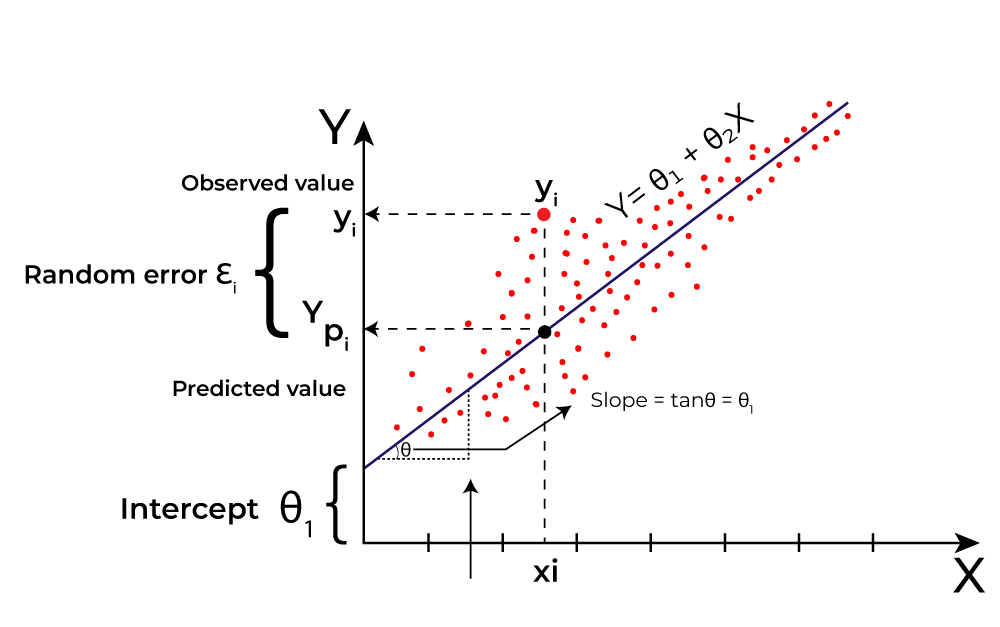
where the slope \(b\) and intercept \(a\) can be computed from summary statistics:
\( \displaystyle b = r\cdot \dfrac{s_y}{s_x}, \qquad a = \bar{y} – b\bar{x} \)
Here \(r\) is the sample correlation, \(s_x,s_y\) are the sample standard deviations, and \(\bar{x},\bar{y}\) are sample means.
How to predict
- Compute \(b\) using \( b = r\,(s_y/s_x)\) (or obtain \(b\) directly from regression output).
- Compute \(a = \bar{y} – b\bar{x}\).
- Substitute the desired \(x\) value into \(\hat{y} = a + b x\) to get the predicted response.
- Optionally compute the residual \( e = y_{\text{obs}} – \hat{y} \) if an observed \(y\) exists.
Interpretation
- Slope \(b\): predicted change in \(y\) for a one–unit increase in \(x\). (Units matter.)
- Intercept \(a\): predicted \(y\) when \(x=0\). Interpret with caution—may be meaningless if \(x=0\) is outside the data range.
- Residual: \( e = y – \hat{y} \). Positive residual → observed above prediction; negative → below.
- Caution: Do not extrapolate predictions far beyond the range of observed \(x\) values.
Example
Data for 5 students (hours studied \(x\), exam score \(y\)):
\( (2,65), (4,70), (5,75), (7,85), (9,95) \).
Use the sample summaries to find the least-squares line and predict the exam score for a student who studies 6 hours. Also compute the residual if a student who studied 7 hours scored 85.
▶️ Answer / Explanation
Step 1 — compute summary statistics (from the data)
\( \bar{x} = 5.4,\quad \bar{y} = 78.0. \)
Sample standard deviations: \( s_x \approx 2.70,\quad s_y \approx 12.04. \)
Correlation: \( r \approx 0.991 \) (very strong positive linear association).
Step 2 — compute slope and intercept
\( b = r\cdot\dfrac{s_y}{s_x} \approx 0.991\cdot\dfrac{12.04}{2.70} \approx 4.42. \)
\( a = \bar{y} – b\bar{x} \approx 78.0 – 4.42(5.4) \approx 54.15. \)
Regression equation (least-squares line):
\( \displaystyle \hat{y} = 54.15 + 4.42x \).
Step 3 — predict for \(x=6\)
\( \hat{y}(6) = 54.15 + 4.42(6) = 54.15 + 26.52 \approx 80.67. \)
Answer: Predicted exam score ≈ 80.7 for a student who studies 6 hours.
Step 4 — residual for the 7-hour student who scored 85
\( \hat{y}(7) = 54.15 + 4.42(7) \approx 85.09. \)
Residual \( e = y_{\text{obs}} – \hat{y} = 85 – 85.09 \approx -0.09 \) (observed is about 0.09 points below prediction).
Interpretation: The slope \(4.42\) means we predict about a 4.42-point increase in exam score for each additional hour studied. The intercept ~54.15 estimates the predicted score at \(x=0\) hours (interpret with caution). The residual near zero for the 7-hour student indicates the model predicted that score well.
Notes & cautions:
- Because the regression was computed from this sample, predicted values have sampling variability.
- Predictions far outside the observed \(x\)-range (here 2–9 hours) are extrapolations and may be unreliable.
- Check residuals and plot to ensure a linear model is appropriate before trusting predictions.
Example
Data summary: A real estate sample shows house size (\(x\), in 1000 sq. ft.) vs price (\(y\), in $1000). Regression output from calculator:
\( a = 50.2,\; b = 120.5,\; r = 0.93. \)
Predict the price of a 2.5-thousand sq. ft. house. How do you get this result quickly on a TI-84?
▶️ Answer / Explanation
Step 1 — TI-84 Regression:
- Enter sizes in L1, prices in L2.
- STAT → CALC → 8:LinReg(ax+b).
- Result: \( a=50.2,\; b=120.5 \).
Step 2 — Prediction:
Equation: \( \hat{y} = 50.2 + 120.5x \).
For \(x=2.5\): \( \hat{y} = 50.2 + 120.5(2.5) = 50.2 + 301.25 = 351.45 \).
Predicted price: ≈ \$351,450.
Step 3 — TI-84 One-line recipe:
After running LinReg(ax+b): type Y1 = a + bX in Y= menu (press VARS → Statistics → EQ → RegEq). Then use 2nd → CALC → value at \(x=2.5\) to get \(\hat{y}\).
Interpretation: Each additional 1000 sq. ft. adds about \$120,500 to the predicted price. A 2.5-thousand sq. ft. house is predicted at ≈ \$351,450.