
2.8.A.1 Random Variable
A random variable is a variable whose value is a numerical outcome resulting from a random process or experiment.
Instead of describing outcomes with words (such as Heads or Tails), a random variable assigns a number to each outcome.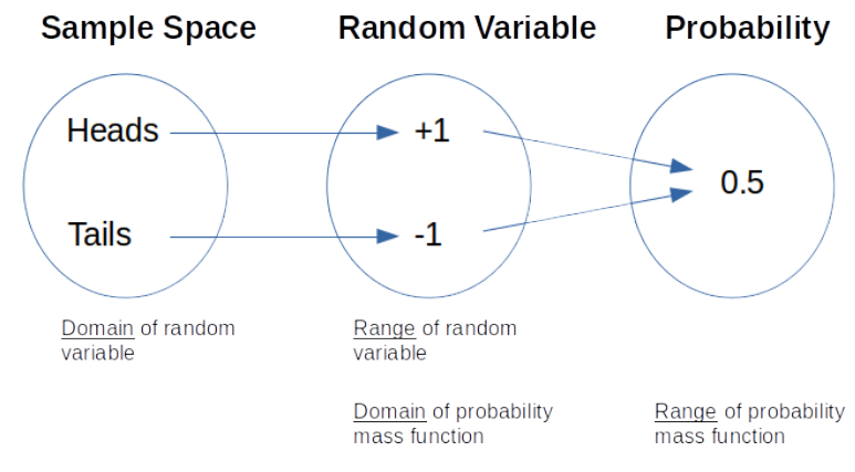
Random variables are usually represented by capital letters such as
\(X,\;Y,\;Z\)
Each possible value of the random variable corresponds to one possible outcome of the random experiment.
Key Idea
A random variable converts the outcomes of a random process into numerical values that can be analyzed using probability and statistics.
Example 1: Tossing Two Coins
Suppose two fair coins are tossed.
Define the random variable
\(X=\) Number of Heads obtained.
| Outcome | Value of \(X\) |
|---|---|
| TT | 0 |
| HT | 1 |
| TH | 1 |
| HH | 2 |
The random variable \(X\) can take only the values
\(0,\;1,\;2\)
Example 2: Rolling a Die
A fair six-sided die is rolled once.
Define the random variable
\(Y=\) Number shown on the die.
| Outcome | Value of \(Y\) |
|---|---|
| 1 | 1 |
| 2 | 2 |
| 3 | 3 |
| 4 | 4 |
| 5 | 5 |
| 6 | 6 |
Characteristics of a Random Variable
- Its values are numerical.
- Its values come from a random experiment.
- Each possible value has an associated probability.
- Random variables are commonly represented by capital letters such as \(X\) or \(Y\).
Random Variable vs. Outcome
| Outcome | Random Variable |
|---|---|
| Actual result of a random experiment. | Numerical value assigned to the outcome. |
| Example: HH | Example: \(X=2\) Heads |
| Example: HT | Example: \(X=1\) Head |
Important AP Exam Notes
- A random variable assigns a numerical value to each outcome of a random process.
- Random variables are usually denoted by capital letters such as \(X\) or \(Y\).
- Each possible value of the random variable has an associated probability.
- Random variables are the foundation for constructing probability distributions.
- In AP Statistics Unit 2, random variables are typically discrete, meaning they take a finite or countable number of values.
Common AP Exam Mistakes
| Incorrect | Correct |
|---|---|
| Confusing the random variable with the actual outcome. | A random variable is the numerical value assigned to an outcome. |
| Using words as the values of a random variable. | Random variables always take numerical values. |
| Thinking a random variable predicts the outcome. | A random variable records the numerical result after the experiment occurs. |
Example
A fair coin is tossed three times.
Define the random variable
\(X=\) Number of Heads obtained.
List all possible values of the random variable \(X\).
▶️ Answer / Explanation
The number of Heads obtained can be
- 0 Heads
- 1 Head
- 2 Heads
- 3 Heads
Therefore, the possible values of the random variable are
\(X=\{0,1,2,3\}\)
Notice that the random variable records the number of Heads, not the individual outcomes such as HHT or TTH.
2.8.A.2 Probability Distribution for a Discrete Random Variable
A probability distribution for a discrete random variable lists every possible value of the random variable along with its corresponding probability.
Each possible value of the random variable has exactly one probability associated with it, and together these probabilities describe how likely each outcome is.
Since one of the possible values must occur, the probabilities of all possible values always add up to \( 1 \)
Properties of a Discrete Probability Distribution
A valid probability distribution must satisfy the following conditions:
- Each probability must satisfy
\( 0 \le P(X=x) \le 1 \)
- The sum of all probabilities must equal
\( \sum P(X=x)=1 \)
- Every possible value of the random variable must be included.
Example 1: Tossing Two Fair Coins
Suppose two fair coins are tossed.
Define the random variable
\(X=\) Number of Heads obtained.
The possible values of \(X\) are
\(0,\;1,\;2\)
The probability distribution is
| \(X\) | \(P(X)\) |
|---|---|
| 0 | \( \frac14 \) |
| 1 | \( \frac24=\frac12 \) |
| 2 | \( \frac14 \) |
| Total | \(1\) |
Notice that
\( \frac14+\frac12+\frac14=1 \)
Therefore, this is a valid probability distribution.
Example 2: Rolling a Fair Die
Let
\(Y=\) Number rolled on a fair six-sided die.
| \(Y\) | \(P(Y)\) |
|---|---|
| 1 | \( \frac16 \) |
| 2 | \( \frac16 \) |
| 3 | \( \frac16 \) |
| 4 | \( \frac16 \) |
| 5 | \( \frac16 \) |
| 6 | \( \frac16 \) |
| Total | \(1\) |
How to Check Whether a Probability Distribution is Valid
- Verify that every probability is between 0 and 1.
- Add all probabilities together.
- If the total equals 1, the distribution is valid.
Important AP Exam Notes
- A probability distribution lists every possible value of a discrete random variable and its probability.
- Every probability must satisfy \(0\le P(X=x)\le1\)
- The probabilities of all possible values must add to \(1\)
- If the probabilities do not sum to 1, the table is not a valid probability distribution.
- Each possible value of the random variable must appear exactly once in the distribution.
Common AP Exam Mistakes
| Incorrect | Correct |
|---|---|
| Probabilities add to 0.95. | They must add to exactly 1. |
| A probability equals 1.20. | Every probability must be between 0 and 1. |
| Leaving out one possible value of the random variable. | Include every possible value. |
Example
A random variable \(X\) has the following probability distribution.
| \(X\) | \(P(X)\) |
|---|---|
| 0 | 0.20 |
| 1 | 0.35 |
| 2 | 0.45 |
Determine whether this is a valid probability distribution.
▶️ Answer / Explanation
Step 1: Check that each probability is between 0 and 1.
All probabilities satisfy this condition.
Step 2: Add the probabilities.
\(0.20+0.35+0.45=1.00\)
Conclusion
Since every probability is between 0 and 1 and the probabilities sum to 1, this is a valid discrete probability distribution.
2.8.A.3 Constructing a Discrete Probability Distribution
A discrete probability distribution can be created by using either the rules of probability or by estimating probabilities with a simulation.
The method used depends on the information available about the random process.
- If the probabilities can be calculated exactly using probability rules, construct the distribution using theoretical probability.
- If calculating the probabilities exactly is difficult or impossible, estimate the probabilities using a simulation.
Method 1: Using the Rules of Probability
When the probabilities of all outcomes are known, use probability rules to calculate the probability for every possible value of the random variable.
Example
A fair coin is tossed twice.
Define
\(X=\) Number of Heads obtained.
The sample space is
\(\{HH,\ HT,\ TH,\ TT\}\)
The probability distribution is
| \(X\) | \(P(X)\) |
|---|---|
| 0 | \( \frac14 \) |
| 1 | \( \frac24=\frac12 \) |
| 2 | \( \frac14 \) |
Method 2: Using a Simulation
When exact probabilities are difficult to determine, perform a simulation by repeating the random process many times.
The estimated probability of each value is
\( \text{Estimated Probability}=\dfrac{\text{Number of Times the Value Occurred}}{\text{Total Number of Simulation Trials}} \)
Example
A simulation of rolling two dice is performed 500 times.
Let
\(X=\) Sum of the two dice.
Suppose a sum of 7 occurs 82 times.
The estimated probability is
\(P(X=7)=\dfrac{82}{500}=0.164\)
Steps for Constructing a Probability Distribution
- Define the random variable.
- List every possible value of the random variable.
- Determine the probability of each value using probability rules or simulation.
- Verify that all probabilities are between 0 and 1.
- Verify that the probabilities sum to 1.
Important AP Exam Notes
- Probability distributions may be constructed using theoretical probability or simulation.
- Simulations estimate probabilities using relative frequencies.
- Larger simulations generally produce more accurate probability estimates.
- Always verify that the completed distribution satisfies the requirements of a valid probability distribution.
Example
A fair die is rolled once.
Define the random variable
\(X=\) Number rolled.
Construct the probability distribution.
▶️ Answer / Explanation
Possible values:
\(1,\ 2,\ 3,\ 4,\ 5,\ 6\)
Since the die is fair, each outcome has probability
\( \frac16 \)
The probability distribution is
| \(X\) | \(P(X)\) |
|---|---|
| 1 | \( \frac16 \) |
| 2 | \( \frac16 \) |
| 3 | \( \frac16 \) |
| 4 | \( \frac16 \) |
| 5 | \( \frac16 \) |
| 6 | \( \frac16 \) |
2.8.A.4 Representing a Discrete Probability Distribution
A discrete probability distribution may be represented in several equivalent ways.
The most common representations are:
- A table
- A graph
- A probability function
Each representation shows the probability associated with every possible value of the random variable.
1. Probability Distribution Table
The table lists every possible value of the random variable together with its probability.
| \(X\) | \(P(X)\) |
|---|---|
| 0 | 0.25 |
| 1 | 0.50 |
| 2 | 0.25 |
2. Probability Distribution Graph
A probability distribution can also be displayed using a bar graph.
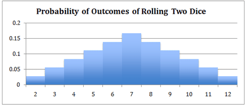
- The horizontal axis shows the values of the random variable.
- The vertical axis shows the probability of each value.
- Each bar represents one possible value of the random variable.
3. Probability Function
A probability distribution may also be written as a function.
Example:
- \(P(X=0)=0.25\)
- \(P(X=1)=0.50\)
- \(P(X=2)=0.25\)
Summary of Representations
| Representation | Description |
|---|---|
| Table | Lists every value and its probability. |
| Graph | Displays probabilities using bars. |
| Function | Defines the probability for each value mathematically. |
Important AP Exam Notes
- The same probability distribution can be represented by a table, graph, or function.
- All representations must contain every possible value of the random variable.
- The probabilities shown must form a valid probability distribution.
- On the AP Exam, probability distributions are most commonly presented using tables and probability histograms (bar graphs).
Example
The probability distribution for a random variable is shown below.
| \(X\) | \(P(X)\) |
|---|---|
| 0 | 0.30 |
| 1 | 0.50 |
| 2 | 0.20 |
Identify two different ways this probability distribution could be represented.
▶️ Answer / Explanation
This probability distribution can be represented as:
- A probability distribution table.
- A probability bar graph (probability histogram).
- A probability function listing \(P(X=x)\) for each value.
Each representation displays the same probabilities for the random variable.
2.8.A.5 Cumulative Probability Distribution
A cumulative probability distribution shows the probability that a discrete random variable is less than or equal to a particular value.
Instead of giving the probability of exactly one value, a cumulative probability distribution adds the probabilities of all values up to and including that value.
The cumulative probability is written as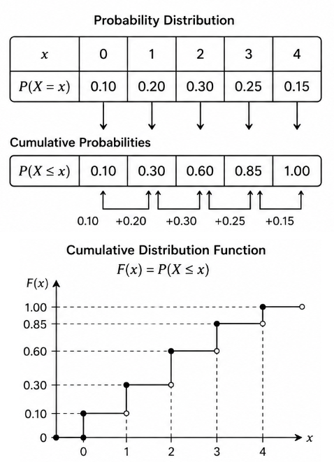
\( P(X\le x) \)
which is read as
“The probability that the random variable \(X\) is less than or equal to \(x\).”
Cumulative Probability Formula
For a discrete random variable, the cumulative probability is calculated by adding the probabilities of all values less than or equal to \(x\).
\( P(X\le x)=\sum P(X=x_i) \)
where the sum includes every value \(x_i\) that satisfies
\( x_i\le x \)
Example 1: Constructing a Cumulative Probability Distribution
Suppose the probability distribution of a random variable \(X\) is given below.
| \(X\) | \(P(X)\) |
|---|---|
| 0 | 0.20 |
| 1 | 0.35 |
| 2 | 0.30 |
| 3 | 0.15 |
The cumulative probability distribution is
| Value | Calculation | Cumulative Probability |
|---|---|---|
| \(P(X\le0)\) | 0.20 | 0.20 |
| \(P(X\le1)\) | 0.20 + 0.35 | 0.55 |
| \(P(X\le2)\) | 0.20 + 0.35 + 0.30 | 0.85 |
| \(P(X\le3)\) | 0.20 + 0.35 + 0.30 + 0.15 | 1.00 |
Example 2
Using the probability distribution above, find
\(P(X\le2)\)
Add the probabilities for all values less than or equal to 2.
\(P(X\le2)=0.20+0.35+0.30=0.85\)
Interpretation:
There is an 85% probability that the value of the random variable is 2 or less.
Representing a Cumulative Probability Distribution
A cumulative probability distribution may be represented as:
- A table listing \(P(X\le x)\) for every value of the random variable.
- A function that gives the cumulative probability for each value of \(x\).
Properties of a Cumulative Probability Distribution
- Cumulative probabilities are always between 0 and 1.
- Cumulative probabilities never decrease; they either increase or remain the same as \(x\) increases.
- The final cumulative probability is always \(1\) because all possible values have been included.
Important AP Exam Notes
- A cumulative probability distribution gives \(P(X\le x)\), not \(P(X=x)\).
- To find a cumulative probability, add all probabilities up to and including the specified value.
- The cumulative probability distribution can be displayed as a table or a function.
- The last cumulative probability must always equal 1.
- Cumulative probabilities never decrease as the random variable increases.
Common AP Exam Mistakes
| Incorrect | Correct |
|---|---|
| Using only \(P(X=x)\). | Add all probabilities for values less than or equal to \(x\). |
| Forgetting to include the specified value. | Remember that “less than or equal to” includes the value itself. |
| Final cumulative probability is not 1. | The last cumulative probability must always equal 1. |
Example
The probability distribution of a random variable \(X\) is shown below.
| \(X\) | \(P(X)\) |
|---|---|
| 0 | 0.10 |
| 1 | 0.25 |
| 2 | 0.40 |
| 3 | 0.25 |
Construct the cumulative probability distribution.
▶️ Answer / Explanation
| Value | Cumulative Probability |
|---|---|
| \(P(X\le0)\) | 0.10 |
| \(P(X\le1)\) | 0.10 + 0.25 = 0.35 |
| \(P(X\le2)\) | 0.35 + 0.40 = 0.75 |
| \(P(X\le3)\) | 0.75 + 0.25 = 1.00 |
The final cumulative probability equals 1, confirming that every possible value has been included.