Estimating Parameters for the Least-Squares Regression Line
The least-squares regression line is the line that minimizes the sum of squared residuals.
The model is written as: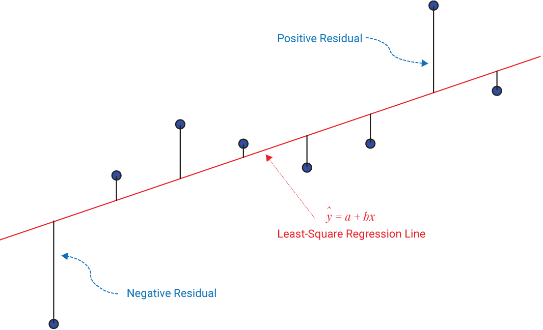
\( \displaystyle \hat{y} = a + b x \)
- \( \hat{y} \): predicted response
- \( a \): intercept
- \( b \): slope
Formulas for Estimating Parameters:
\( \displaystyle b = r \cdot \dfrac{s_y}{s_x}, \quad a = \bar{y} – b\bar{x} \)
- \(r\): correlation between \(x\) and \(y\)
- \(s_x, s_y\): standard deviations of \(x\) and \(y\)
- \(\bar{x}, \bar{y}\): means of \(x\) and \(y\)
Interpreting Coefficients:
- Slope \(b\): The predicted change in the response variable \(y\) for a one-unit increase in the explanatory variable \(x\).
- Intercept \(a\): The predicted value of \(y\) when \(x=0\). This may or may not be meaningful, depending on the context.
Cautions:
- Interpret slope only within the observed range of data.
- Do not extrapolate predictions for \(x\)-values far outside the data.
- The regression line summarizes association, not causation.
Example
A dataset records students’ hours studied (\(x\)) and exam scores (\(y\)).
Summary statistics:
- \( \bar{x} = 5,\; s_x = 2 \)
- \( \bar{y} = 70,\; s_y = 10 \)
- Correlation \( r = 0.8 \)
Find the least-squares regression line equation.
▶️ Answer / Explanation
\( b = r \cdot \dfrac{s_y}{s_x} = 0.8 \cdot \dfrac{10}{2} = 4.0 \).
\( a = \bar{y} – b\bar{x} = 70 – 4(5) = 50 \).
Regression Equation: \( \hat{y} = 50 + 4x \).
Example
Suppose the regression line is \( \hat{y} = 50 + 4x \), where \(x\) = hours studied and \(y\) = exam score.
Interpret the slope and intercept in context.
▶️ Answer / Explanation
Slope (4): For each additional hour of study, the model predicts an average increase of 4 exam points.
Intercept (50): When \(x=0\) (a student does not study at all), the model predicts an exam score of 50. This interpretation makes sense here, since “0 hours” is within the possible range.
The Coefficient of Determination (\( r^2 \))
In simple linear regression, \( r^2 \) is the square of the correlation coefficient \( r \). It is called the coefficient of determination.
Formula: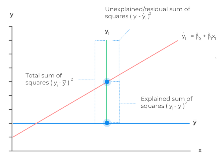
\( \displaystyle r^2 = \dfrac{\text{Explained Variation}}{\text{Total Variation}} \)
$\rm R^2 = \frac{\text{Explained Variation}}{\text{Total Variation}} = \frac{\text{Sum of Squares Regression (SSR)}}{\text{Sum of Squares Total (SST)}}$
$\text{Intuitively we can think of the above formula as:}$
$\rm R^2 = \frac{\text{Total Variation}-\text{Unexplained Variation}}{\text{Total Variation}} $
$\frac{\text{Sum of Squares Total (SST)}-\text{Sum of Squared Errors (SSE)}}{\text{Sum of Squares Total}}$
$\text{Simplifying the above formula gives:}$
$\rm R^2 = 1 – \frac{\text{Sum of Squared Errors (SSE)}}{\text{Sum of Squares Total (SST)}}$
Interpretation:
\( r^2 \) represents the proportion of variation in the response variable (\(y\)) that is explained by the explanatory variable (\(x\)) in the regression model.
- Values of \( r^2 \) range from 0 to 1:
- \( r^2 = 0 \): The model explains none of the variation.
- \( r^2 = 1 \): The model explains all of the variation.
- Intermediate values: Higher \( r^2 \) means better explanatory power.
- \( r^2 \) alone does not indicate whether the model is appropriate (check residual plots).
Example
Suppose the correlation between hours studied (\(x\)) and exam scores (\(y\)) is \( r = 0.8 \).
What does \( r^2 \) tell us in this context?
▶️ Answer / Explanation
Step 1 — compute \( r^2 \):
\( r^2 = (0.8)^2 = 0.64 \).
Step 2 — interpret:
About 64% of the variation in exam scores can be explained by a linear relationship with hours studied. The remaining 36% of the variation is due to other factors (or random variation).
Note: A strong \( r^2 \) does not prove causation. Other variables could also influence exam scores.
Example:
An analyst determines that \(\displaystyle \sum_{i=1}^{6} (Y_i – \bar{Y})^2 = 0.0013844\) and \(\displaystyle \sum_{i=1}^{6} (Y_i – \hat{Y})^2 = 0.0003206\) from a regression analysis of inflation on unemployment. Find the coefficient of determination \((R^2)\).
▶️ Answer / Explanation
\(\displaystyle R^2 = \dfrac{\text{SST} – \text{SSE}}{\text{SST}}\)
- SST = Total Sum of Squares = \(\displaystyle \sum (Y_i – \bar{Y})^2\)
- SSE = Sum of Squared Errors = \(\displaystyle \sum (Y_i – \hat{Y})^2\)
\(\displaystyle R^2 = \dfrac{0.0013844 – 0.0003206}{0.0013844}\)
\(\displaystyle R^2 = \dfrac{0.0010638}{0.0013844} \approx 0.7684\)
Final Answer: \(R^2 \approx 0.7684 = 76.84\%\)
About 76.8% of the variation in unemployment is explained by inflation in this model.