Identifying Influential Points in Regression
An influential point is an observation that, if removed, would significantly change the slope, intercept, or correlation of the regression line. Influential points often lie far away in the x-direction (explanatory variable), giving them large leverage on the regression model.
Key Characteristics: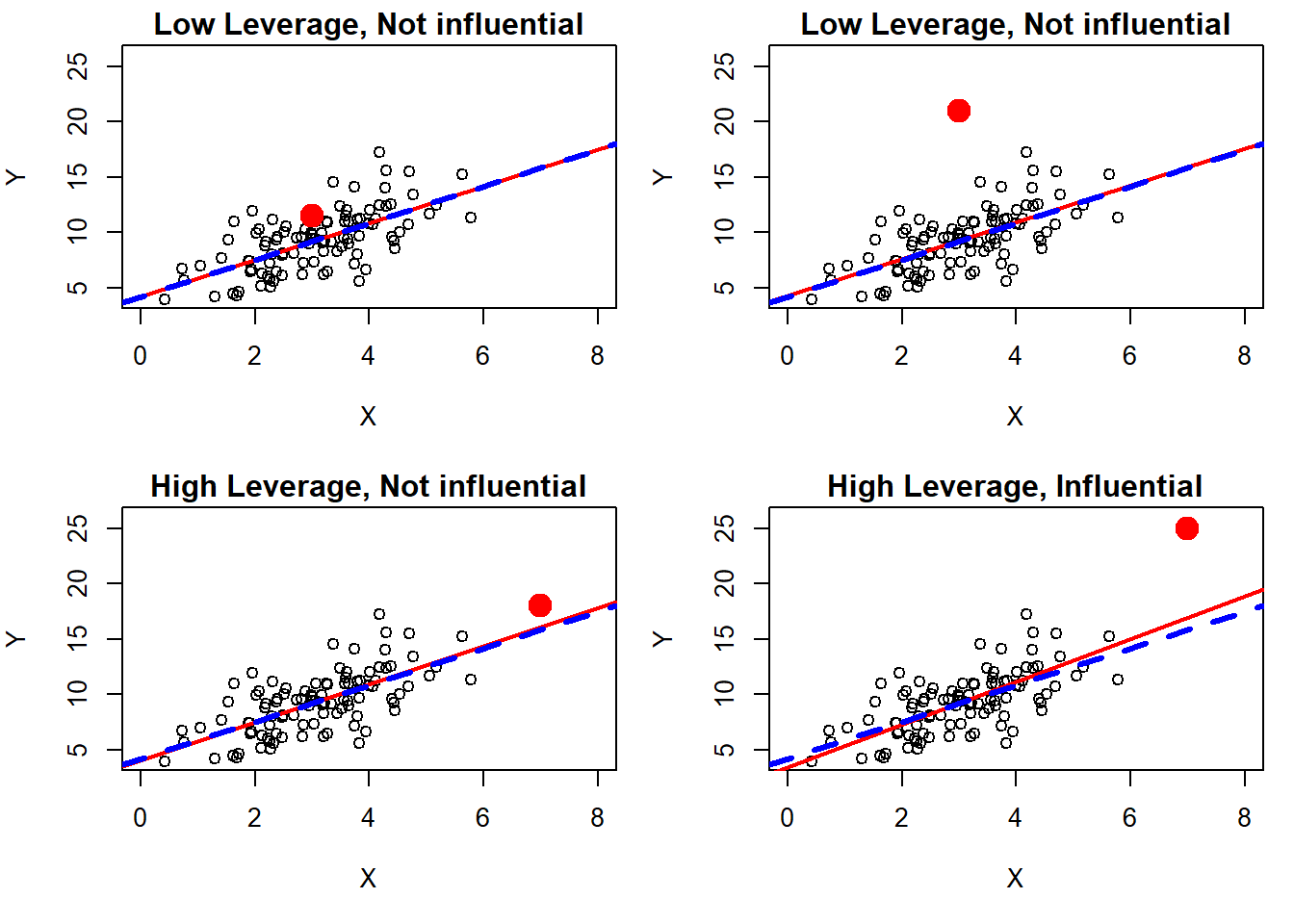
- Influential points are not just outliers in the \(y\)-direction. They are usually extreme in the \(x\)-direction.
- An outlier in \(y\) may or may not be influential. Its influence depends on how much it changes the regression line.
Removing an influential point can drastically change:
- The slope of the regression line
- The \( y \)-intercept
- The correlation coefficient \( r \)
- The coefficient of determination \( r^2 \)
How to Identify:
- Plot the data with and without the point. If the regression line changes noticeably, the point is influential.
- Look for points far out in the \(x\)-direction (high leverage points).
- Use residual plots: unusually large residuals or leverage suggest possible influence.
Example
A scatterplot relates study hours (\(x\)) to test score (\(y\)). Most students studied between 2 and 8 hours. One student studied 20 hours and scored 85.
Is this student’s data point likely influential?
▶️ Answer / Explanation
Yes. The student’s value is far in the \(x\)-direction (20 hours), much larger than the rest of the data. Because it is far away in the explanatory variable, it has high leverage. This point could pull the regression line upward and increase the slope, making it an influential point.
Example
Data relate house size (\(x\), in square feet) to sale price (\(y\), in dollars). One small house (800 sq ft) sold for $\$2$ million, while most houses sold between $\$200,000$ and $\$500,000$.
Is this point influential?
▶️ Answer / Explanation
No. This point is unusual in the \(y\)-direction (a vertical outlier) but not in the \(x\)-direction, since its house size is within the range of other data. It may be an outlier, but it is not influential, because removing it would not dramatically change the slope of the regression line.
Predictions with Transformed Regression
Sometimes, data are transformed to make the relationship linear, stabilize variance, or normalize residuals. Common transformations include:
- Logarithmic: \( y’ = \log(y) \) or \( x’ = \log(x) \)

- Square root: \( y’ = \sqrt{y} \)
- Reciprocal: \( y’ = 1/y \) or \( x’ = 1/x \)
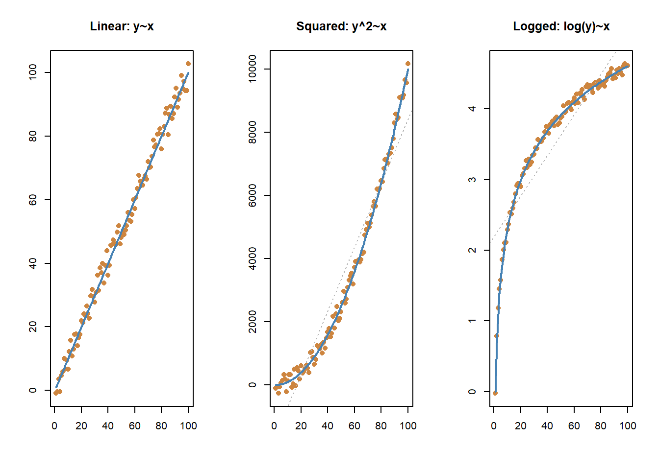
The regression line is then fit to the transformed variables:
\( \displaystyle \hat{y}’ = a + b x’ \)
where \(y’\) and/or \(x’\) are transformed values.
Steps to Predict the Response:
- Transform the explanatory variable \(x\) as specified (e.g., \( x’ = \log(x) \)).
- Use the regression equation on the transformed scale to calculate \( \hat{y}’ = a + b x’ \).
- Back-transform the predicted response to the original scale if necessary (e.g., \( \hat{y} = 10^{\hat{y}’} \) if log base 10 was used).
- Interpret the result in the context of the original variables.
Cautions:
- Always back-transform predictions to the original scale when interpreting.
- Check whether the transformation makes sense for the context (e.g., cannot take log of negative values).
- Residuals should be examined on the transformed scale to validate the model.
Example
Researchers measured bacterial population (\(y\)) over time (\(x\)) and found an exponential growth pattern. They transformed \(y\) using logarithms: \( y’ = \log_{10}(y) \).
Regression equation on transformed data: \( \hat{y}’ = 0.3 + 0.2x \)
Predict the population at \(x = 10\) hours.
▶️ Answer / Explanation
Step 1 — apply the regression equation on transformed scale:
\( \hat{y}’ = 0.3 + 0.2(10) = 0.3 + 2 = 2.3 \)
Step 2 — back-transform to original scale:
\( \hat{y} = 10^{\hat{y}’} = 10^{2.3} \approx 199.5 \)
Step 3 — interpretation:
The model predicts approximately 200 bacteria at 10 hours.
Note: Predictions are meaningful only within the range of observed \(x\) values. The log transformation ensures linearity and stabilizes variance in this example.