Question 1
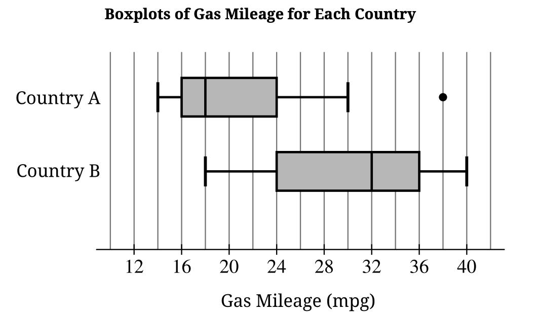
i. What is the range of the combined data set? Justify your answer.
ii. What is a possible value of the median of the combined data set? Justify your answer by referencing the boxplots shown.
Most-appropriate topic codes (CED):
• TOPIC 1.10: Mean vs Median (Skewness) — part (b)
▶️ Answer/Explanation
(A)
• Center: Median of B (~32 mpg) > Median of A (18 mpg).
• Spread: Range of A (24 mpg) > Range of B (22 mpg). IQR of B > IQR of A .
• Shape/Outliers: Country A is right-skewed with a high outlier. Country B is roughly symmetric.
(B)
Greater than 18 mpg.
The distribution for Country A is skewed to the right. In a right-skewed distribution, the mean is pulled toward the tail, making it greater than the median (18) .
(C)(i)
26 mpg.
Range = Combined Max – Combined Min.
Max is from Country B (40). Min is from Country A (14).
\(40 – 14 = 26\) mpg .
(C)(ii)
24 mpg.
The combined sample has 200 cars. The median is the average of the 100th and 101st values.
Q3 of Country A is 24 (75% of 100 \(\le\) 24). Q1 of Country B is 24 (25% of 100 \(\le\) 24).
Thus, ~100 values are \(\le 24\) and ~100 values are \(\ge 24\), so the median is 24 .
Question 2
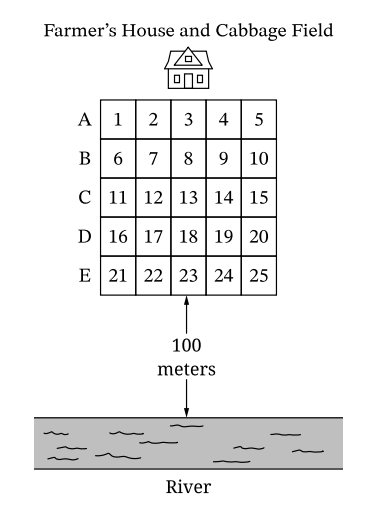
Sampling method I: Select region 3, which is closest to the farmer’s house and farthest from the river. Examine every cabbage plant in the region for aphid damage.
Sampling method II: Randomly select one row (A, B, C, D, or E). For every region in the selected row, examine every cabbage plant for aphid damage.
Sampling method III: Randomly select one region from each of rows A, B, C, D, and E. For each selected region, examine every cabbage plant for aphid damage.
Most-appropriate topic codes (CED):
• TOPIC 3.3: Potential Sources of Bias — part (b)
▶️ Answer/Explanation
(A)
Not appropriate.
It is a convenience sample. Region 3 is farthest from the river. If damage is related to the river, this region will likely have less damage than the field average, leading to an underestimate .
(B)
Overestimate.
Row E is closest to the river. If the farmer’s belief is correct (damage is greater near the river), the proportion of damaged plants in Row E will be higher than the true population proportion .
(C)
Stratified Sampling Procedure:
1. Label regions 1-5 in Row A.
2. Randomly select one number (1-5) using a random number generator.
3. Repeat independently for Rows B, C, D, and E (selecting one region from each row).
4. Examine all plants in the 5 selected regions .
Question 3
ii. Suppose two songs are selected at random to be played. What is the probability that both songs are rock songs? Show your work.
i. Define the random variable of interest to Ms. Fey, and state how the random variable is distributed.
ii. What is the expected value for the random variable in part B (i)? Show your work.
i. Determine the probability that 4 or more rock songs in a particular one-hour period will be played. Show your work.
ii. Suppose 4 rock songs are played during a particular one-hour period. Does this provide strong evidence that the song selection process was not truly random? Justify your answer without performing an inference procedure.
Most-appropriate topic codes (CED):
• TOPIC 4.10: Binomial Distribution — part (b)
▶️ Answer/Explanation
(A)(i)
\(P(\text{Rock}) = \frac{100}{1000} = 0.10\) .
(A)(ii)
\(P(\text{Both Rock}) = 0.10 \times 0.10 = 0.01\) (Independent events) .
(B)(i)
Let \(X\) = # of rock songs in 20.
Distribution: Binomial with \(n=20\), \(p=0.10\) .
(B)(ii)
\(E(X) = np = 20(0.10) = 2\) rock songs .
(C)(i)
\(P(X \ge 4) = 1 – P(X \le 3)\)
\(P(X \ge 4) = 1 – 0.867 = 0.133\) .
(C)(ii)
No.
\(P(\ge 4 \text{ rock songs}) = 13.3\%\). This is not small enough (< 5%) to be significant evidence against randomness .
Question 4
Most-appropriate topic codes (CED):
▶️ Answer/Explanation
State: We will test \(H_0: p = 0.22\) versus \(H_a: p > 0.22\) at \(\alpha = 0.05\), where \(p\) is the true proportion of students at Karen’s school who use the app weekly.
Plan: One-sample z-test for proportion.
Conditions:
• Random: Simple random sample of 130 students (stated).
• 10% Condition: \(130 < 10\%\) of 2,000+ students (satisfied).
• Large Counts: \(np_0 = 130(0.22) = 28.6 \ge 10\) and \(n(1-p_0) = 130(0.78) = 101.4 \ge 10\) (satisfied).
Do:
Sample proportion \(\hat{p} = \frac{38}{130} \approx 0.2923\).
Test statistic \(z = \frac{\hat{p} – p_0}{\sqrt{\frac{p_0(1-p_0)}{n}}} = \frac{0.2923 – 0.22}{\sqrt{\frac{0.22(0.78)}{130}}} \approx \frac{0.0723}{0.0363} \approx 1.99\).
P-value \(P(Z > 1.99) \approx 0.0233\).
Conclude:
Since the p-value (\(0.0233\)) is less than \(\alpha\) (\(0.05\)), we reject \(H_0\). [cite_start]There is convincing statistical evidence to support Karen’s belief that the proportion of students at her school who use the app is greater than \(0.22\) [cite: 379-384].
Question 5
| Number of Bedrooms | 1 | 2 | 3 | 4 | 5 | 6 |
|---|---|---|---|---|---|---|
| Proportion of Houses | 0.12 | 0.22 | 0.28 | 0.22 | 0.14 | 0.02 |
i. A house from the sample will be selected at random. What is the probability that the house had fewer than 3 bedrooms? Show your work.
ii. What is the mean number of bedrooms for the sample of newly built houses in 2024? Show your work.
i. In the context of Rodney’s investigation, state the hypotheses for the test.
ii. Explain, in context, what a Type I error would be for Rodney’s hypothesis test.
Most-appropriate topic codes (CED):
• TOPIC 7.2: One-Sample t-Test for Mean — part (b)
• TOPIC 7.4: Confidence Intervals for Mean — part (c)
▶️ Answer/Explanation
(A)(i)
\(P(\text{< 3}) = P(1) + P(2) = 0.12 + 0.22 = 0.34\).
(A)(ii)
Mean \(\bar{x} = \sum x_i p_i\)
\(= 1(0.12) + 2(0.22) + 3(0.28) + 4(0.22) + 5(0.14) + 6(0.02)\)
\(= 0.12 + 0.44 + 0.84 + 0.88 + 0.70 + 0.12 = 3.10\).
(B)(i)
\(H_0: \mu = 2.9\) (Mean is 2.9).
\(H_a: \mu \ne 2.9\) (Mean is different from 2.9).
(B)(ii)
Type I error: Concluding that the mean number of bedrooms in 2024 is different from 2.9 when, in reality, it is still 2.9.
(C)
Reject \(H_0\).
The 97% confidence interval is \((3.01, 3.19)\). Since the null value \(2.9\) is not included in the interval, there is convincing evidence at \(\alpha = 0.03\) (\(1 – 0.97\)) that the mean is different from 2.9.
Question 6
Table 1: Summary Statistics of Reading Scores
| n | Mean | Standard Deviation | |
|---|---|---|---|
| 9 a.m. | 50 | 15.2 | 4.12 |
| 3 p.m. | 50 | 17.9 | 4.43 |
\(H_0: \mu_{AM} = \mu_{PM}\)
\(H_a: \mu_{AM} \ne \mu_{PM}\)
i. Calculate Cohen’s d coefficient for Stefan’s study. Show your work.
ii. Higher values of Cohen’s d indicate greater practical importance and lower values of Cohen’s d indicate less practical importance. Typically, we use the intervals listed in Table 2 to help interpret practical importance.
Table 2: Guidelines for Interpreting Cohen’s d Coefficient
| Cohen’s d Coefficient | Practical Importance |
|---|---|
| \(0 \le d \le 0.20\) | Not very meaningful in real life |
| \(0.20 < d < 0.80\) | Somewhat meaningful in real life |
| \(d \ge 0.80\) | Very meaningful in real life |
i. Would the Cohen’s d coefficient in this new situation be smaller than, larger than, or the same as the Cohen’s d coefficient calculated in part C (i)? Explain your answer.
ii. Does the Cohen’s d coefficient described in part D (i) indicate that Stefan’s observed difference in the means in the new situation would have more practical importance than, less practical importance than, or the same practical importance as what was originally determined in part C (ii)? Explain your answer.
Most-appropriate topic codes (CED):
• TOPIC 1.1: Analyzing Quantitative Data — part (c), (d)
▶️ Answer/Explanation
(A)
Reject \(H_0\).
The p-value \((0.002) < \alpha (0.05)\). There is convincing evidence that the mean reading score for children reading at 9 a.m. is different from the mean score for children reading at 3 p.m.
(B)
Independent groups.
A two-sample t-test is used because the data comes from two independent groups of children (randomly assigned). A paired t-test requires matched pairs or the same subject measured twice.
(C)(i)
\(s_p = \sqrt{\frac{4.12^2 + 4.43^2}{2}} \approx \sqrt{18.297} \approx 4.278\).
\(d = \frac{|15.2 – 17.9|}{4.278} = \frac{2.7}{4.278} \approx 0.63\).
(C)(ii)
Somewhat meaningful.
Since \(d \approx 0.63\) is between \(0.20\) and \(0.80\), the result is considered somewhat meaningful in real life.
(D)(i)
Smaller.
Increasing \(s_1\) and \(s_2\) increases the denominator \((s_p)\). With the same numerator (difference in means), a larger denominator results in a smaller \(d\).
(D)(ii)
Less practical importance.
A smaller \(d\) moves closer to 0, indicating less practical importance according to Table 2.