
3.2.A.1 Mean and Standard Deviation of the Sampling Distribution of a Sample Proportion
When random samples of the same size are repeatedly selected from a population, each sample has its own sample proportion \( \hat{p} \).
- The collection of all possible values of \( \hat{p} \) forms the sampling distribution of the sample proportion.
- If the sampled values are independent, then the sampling distribution has a predictable mean and standard deviation.
The mean of the sampling distribution equals the population proportion, while the standard deviation measures how much the sample proportions vary from sample to sample.
Formulas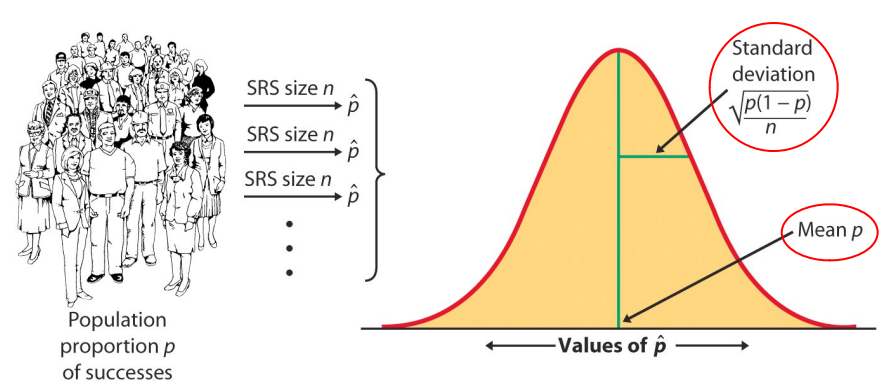
Mean of the Sampling Distribution:
\( \mu_{\hat{p}} = p \)
Standard Deviation of the Sampling Distribution:
\( \sigma_{\hat{p}}=\sqrt{\dfrac{p(1-p)}{n}} \)
Where:
- \( \mu_{\hat{p}} \) = Mean of the sampling distribution of the sample proportion
- \( \sigma_{\hat{p}} \) = Standard deviation of the sampling distribution of the sample proportion
- \( p \) = Population proportion
- \( n \) = Sample size
Key Terms Definition
| Term | Definition |
|---|---|
| Sampling Distribution | The distribution of a statistic obtained from all possible random samples of the same size. |
| Sample Proportion (\( \hat{p} \)) | The proportion of successes in a sample. |
| Mean of the Sampling Distribution | The average of all possible sample proportions; equal to the population proportion \(p\). |
| Standard Deviation of the Sampling Distribution | Measures the variability of the sample proportions from sample to sample. |
Properties of the Sampling Distribution
| Property | Result |
|---|---|
| Mean | \( \mu_{\hat{p}}=p \) |
| Standard Deviation | \( \sigma_{\hat{p}}=\sqrt{\dfrac{p(1-p)}{n}} \) |
| Effect of Increasing Sample Size | Standard deviation decreases, so sample proportions become less variable. |
Example 1
A population has a proportion of homeowners equal to
\( p=0.60 \)
A random sample of
\( n=100 \)
is selected.
Step 1: Calculate the mean.
\( \mu_{\hat{p}}=p=0.60 \)
Step 2: Calculate the standard deviation.
\( \sigma_{\hat{p}}=\sqrt{\dfrac{0.60(1-0.60)}{100}} \)
\(=\sqrt{\dfrac{0.24}{100}}=\sqrt{0.0024}\approx0.049\)
Conclusion:
The sampling distribution has a mean of 0.60 and a standard deviation of approximately 0.049.
Example 2
A population proportion is
\( p=0.25 \)
A random sample of
\( n=400 \)
is selected.
Mean
\( \mu_{\hat{p}}=0.25 \)
Standard Deviation
\( \sigma_{\hat{p}}=\sqrt{\dfrac{0.25(0.75)}{400}}\approx0.022 \)
Important AP Exam Notes
- The mean of the sampling distribution of \( \hat{p} \) is always equal to the population proportion \(p\).
- The standard deviation is calculated using the population proportion, not the sample proportion.
- The formulas apply when the sampled values are independent.
- As the sample size increases, the standard deviation becomes smaller.
- A smaller standard deviation means less variability among sample proportions.
Common AP Exam Mistakes
| Incorrect | Correct |
|---|---|
| Using \( \hat{p} \) instead of \( p \) in the standard deviation formula. | Always use the population proportion \(p\). |
| Thinking the mean equals \( \hat{p} \). | The mean of the sampling distribution equals the population proportion \(p\). |
| Believing larger samples increase variability. | Larger samples decrease the standard deviation. |
Example
A manufacturing company knows that 18% of its products are defective.
A simple random sample of 225 products is selected.
Calculate the mean and standard deviation of the sampling distribution of the sample proportion of defective products.
▶️ Answer / Explanation
Step 1: Calculate the mean.
\( \mu_{\hat{p}}=p=0.18 \)
Step 2: Calculate the standard deviation.
\( \sigma_{\hat{p}}=\sqrt{\dfrac{0.18(1-0.18)}{225}} \)
\(=\sqrt{\dfrac{0.1476}{225}}=\sqrt{0.000656}\approx0.0256\)
Answer
The sampling distribution has
- Mean: \(0.18\)
- Standard deviation: \(0.0256\)
3.2.B.1 Conditions for Sampling Without Replacement
When calculating probabilities involving the sampling distribution of a sample proportion, the observations must be independent.
If sampling is done without replacement, independence is achieved only when both of the following conditions are satisfied: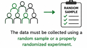
- Randomization Condition — The data must be collected using a random sample or a properly randomized experiment.
- 10% Condition — The population size must be at least 10 times larger than the sample size.
These conditions ensure that selecting one individual does not significantly affect the probability of selecting another individual.
10% Condition
The sample size must satisfy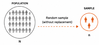
\( n \leq 0.10N \)
Where:
- \( n \) = Sample size
- \( N \) = Population size
Why Are These Conditions Important?
| Condition | Purpose |
|---|---|
| Randomization Condition | Helps ensure the sample is representative of the population and observations are randomly selected. |
| 10% Condition | Allows observations to be treated as approximately independent when sampling without replacement. |
Example 1: Conditions Are Satisfied
A school has 2,500 students.
A simple random sample of 150 students is selected without replacement.
Step 1: Check the Randomization Condition.
The sample is a simple random sample, so the condition is satisfied.
Step 2: Check the 10% Condition.
\(0.10N=0.10(2500)=250\)
Since
\(150\le250\)
the 10% Condition is satisfied.
Conclusion:
Both conditions are met, so the observations may be treated as approximately independent.
Example 2: 10% Condition Fails
A company has 300 employees.
A random sample of 80 employees is selected without replacement.
Calculate 10% of the population.
\(0.10(300)=30\)
Since
\(80>30\)
the sample exceeds 10% of the population.
Conclusion:
The 10% Condition is not satisfied, so independence cannot be assumed.
Important AP Exam Notes
- The Randomization Condition requires that the sample be selected randomly.
- The 10% Condition is required only when sampling without replacement.
- If sampling is done with replacement, observations are automatically independent.
- Always check both conditions before using the sampling distribution of a sample proportion.
- On the AP Exam, you should explicitly state that both conditions are satisfied before performing calculations.
Common AP Exam Mistakes
| Incorrect | Correct |
|---|---|
| Checking only the 10% Condition. | Verify both the Randomization Condition and the 10% Condition. |
| Using the 10% Condition for sampling with replacement. | The 10% Condition is only needed when sampling without replacement. |
| Using \(n\ge0.10N\). | The correct condition is \(n\le0.10N\). |
Example
A city has a population of 12,000 households.
A simple random sample of 900 households is selected without replacement to estimate the proportion that recycle regularly.
Determine whether the conditions required for independence are satisfied.
▶️ Answer / Explanation
Step 1: Check the Randomization Condition.
The sample is a simple random sample, so this condition is satisfied.
Step 2: Check the 10% Condition.
\(0.10(12,000)=1,200\)
Since
\(900\le1,200\)
the 10% Condition is satisfied.
Answer
Both conditions are met, so the observations may be treated as independent.
3.2.B.2 Large Counts Condition for the Sampling Distribution of a Sample Proportion
After verifying that the observations are independent, the next step is to determine whether the sampling distribution of the sample proportion can be modeled using a Normal distribution.
The sampling distribution of the sample proportion \( \hat{p} \) is approximately Normal when the expected number of successes and the expected number of failures are both sufficiently large.
This requirement is called the Large Counts Condition.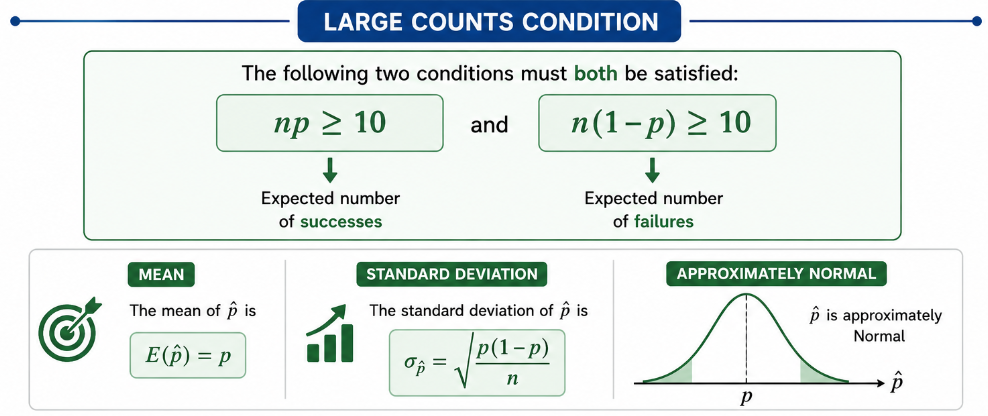
Large Counts Condition
The following two conditions must both be satisfied:
\( np \ge 10 \) and \( n(1-p) \ge 10 \)
Where:
- \( n \) = Sample size
- \( p \) = Population proportion
- \( np \) = Expected number of successes
- \( n(1-p) \) = Expected number of failures
When both conditions are met, the sampling distribution of \( \hat{p} \) is approximately Normal, allowing Normal probability calculations to be used.
Summary of the Condition
| Requirement | Purpose |
|---|---|
| \( np \ge 10 \) | Ensures enough expected successes. |
| \( n(1-p) \ge 10 \) | Ensures enough expected failures. |
| Both conditions satisfied | The sampling distribution of \( \hat{p} \) is approximately Normal. |
Example 1: Large Counts Condition Is Satisfied
A population has a proportion of \( p=0.40 \)
A random sample of \( n=100 \) is selected.
Step 1: Calculate the expected number of successes.
\( np=100(0.40)=40 \)
Step 2: Calculate the expected number of failures.
\( n(1-p)=100(0.60)=60 \)
Since
\(40\ge10\) and \(60\ge10\)
both conditions are satisfied.
Conclusion:
The sampling distribution of \( \hat{p} \) can be approximated by a Normal distribution.
Example 2: Large Counts Condition Is Not Satisfied
A population proportion is \( p=0.04 \)
A sample of \( n=100 \) is selected.
Step 1:
\( np=100(0.04)=4 \)
Step 2:
\( n(1-p)=100(0.96)=96 \)
Since
\(4<10\)
the Large Counts Condition is not satisfied.
Conclusion:
The sampling distribution of \( \hat{p} \) should not be modeled using a Normal distribution.
Important AP Exam Notes
- The Large Counts Condition is used to determine whether the sampling distribution of \( \hat{p} \) is approximately Normal.
- Always verify both \( np\ge10 \) and \( n(1-p)\ge10 \).
- The values \( np \) and \( n(1-p) \) represent the expected numbers of successes and failures.
- If either condition is not satisfied, do not use the Normal model for the sampling distribution of \( \hat{p} \).
- On the AP Exam, clearly show both calculations before stating that the Normal approximation is appropriate.
Common AP Exam Mistakes
| Incorrect | Correct |
|---|---|
| Checking only \(np\). | Both \(np\) and \(n(1-p)\) must be at least 10. |
| Using the sample proportion \( \hat{p} \) instead of the population proportion \(p\) when checking the condition. | Use the population proportion \(p\) (or the hypothesized value in inference problems). |
| Assuming every sampling distribution is Normal. | The Normal approximation is valid only when the Large Counts Condition is satisfied. |
Example
A researcher knows that 30% of adults in a city commute by public transportation.
A simple random sample of 40 adults is selected.
Determine whether the sampling distribution of the sample proportion can be approximated by a Normal distribution.
▶️ Answer / Explanation
Step 1: Calculate the expected number of successes.
\( np=40(0.30)=12 \)
Step 2: Calculate the expected number of failures.
\( n(1-p)=40(0.70)=28 \)
Since \(12\ge10\) and \(28\ge10\)
both conditions are satisfied.
Answer
The sampling distribution of the sample proportion can be approximated by a Normal distribution because both Large Counts conditions are met.