
3.9.A.1 Mean and Standard Deviation of the Sampling Distribution for the Difference Between Two Sample Proportions
Suppose two independent populations have population proportions \(p_1\) and \(p_2\).
If independent random samples are selected from the two populations, the difference between the sample proportions,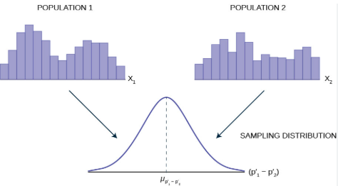
\(\hat{p}_1-\hat{p}_2\)
has its own sampling distribution.
The sampling distribution describes how the difference in sample proportions varies from sample to sample.
Mean of the Sampling Distribution
The mean (expected value) of the sampling distribution is equal to the difference between the two population proportions.
\(\boxed{\mu_{\hat{p}_1-\hat{p}_2}=p_1-p_2}\)
This means that, on average, the difference in the sample proportions equals the true difference in the population proportions.
Standard Deviation of the Sampling Distribution
The standard deviation measures the variability of the differences between sample proportions from one sample to another.
\(\boxed{\sigma_{\hat{p}_1-\hat{p}_2}=\sqrt{\dfrac{p_1(1-p_1)}{n_1}+\dfrac{p_2(1-p_2)}{n_2}}}\)
Mean
\(\mu_{\hat{p}_1-\hat{p}_2}=p_1-p_2\)
Standard Deviation
\(\sigma_{\hat{p}_1-\hat{p}_2}=\sqrt{\dfrac{p_1(1-p_1)}{n_1}+\dfrac{p_2(1-p_2)}{n_2}}\)
Where:
- \(p_1\) = Population proportion for Population 1
- \(p_2\) = Population proportion for Population 2
- \(n_1\) = Sample size from Population 1
- \(n_2\) = Sample size from Population 2
- \(\hat{p}_1\) = Sample proportion from Population 1
- \(\hat{p}_2\) = Sample proportion from Population 2
Interpretation
- The mean tells us where the sampling distribution is centered.
- The standard deviation tells us how much the differences in sample proportions vary from sample to sample.
- A larger standard deviation means greater sampling variability.
- A smaller standard deviation means the sample proportions are more consistent.
Example
A researcher compares the proportion of students who pass an AP Statistics exam at two different schools.
- School A: \(p_1=0.72,\; n_1=150\)
- School B: \(p_2=0.65,\; n_2=180\)
Step 1: Calculate the mean.
\(\mu_{\hat{p}_1-\hat{p}_2}=0.72-0.65=0.07\)
The sampling distribution is centered at 0.07.
Step 2: Calculate the standard deviation.
\(\sigma_{\hat{p}_1-\hat{p}_2}=\sqrt{\dfrac{0.72(0.28)}{150}+\dfrac{0.65(0.35)}{180}}\)
\(=\sqrt{0.001344+0.001264}\)
\(=\sqrt{0.002608}\approx0.051\)
Interpretation
The average difference in sample proportions is expected to be 0.07, with a standard deviation of approximately 0.051.
Effect of Sample Size
| If… | Effect on Standard Deviation |
|---|---|
| Sample sizes increase | Standard deviation decreases. |
| Sample sizes decrease | Standard deviation increases. |
This means larger samples produce more consistent estimates of the difference between population proportions.
Important AP Exam Notes
- The sampling distribution is based on independent random samples.
- The mean of the sampling distribution is \(p_1-p_2\).
- The standard deviation is calculated using the population proportions and sample sizes.
- Larger sample sizes decrease the standard deviation.
- Do not confuse the population proportions (\(p_1,p_2\)) with the sample proportions (\(\hat{p}_1,\hat{p}_2\)).
Common AP Exam Mistakes
| Incorrect | Correct |
|---|---|
| Using \(\hat{p}\) values in the standard deviation formula for a sampling distribution. | Use the population proportions \(p_1\) and \(p_2\). |
| Subtracting sample sizes. | Sample sizes appear in the denominators of the formula. |
| Using \(p_2-p_1\) when the problem defines \(p_1-p_2\). | Always keep the order consistent throughout the problem. |
Example
Two independent populations have the following population proportions:
- \(p_1=0.60,\; n_1=200\)
- \(p_2=0.45,\; n_2=250\)
Calculate the mean and standard deviation of the sampling distribution of \(\hat{p}_1-\hat{p}_2\).
▶️ Answer / Explanation
Mean
\(\mu_{\hat{p}_1-\hat{p}_2}=0.60-0.45=0.15\)
Standard Deviation
\(\sigma_{\hat{p}_1-\hat{p}_2}=\sqrt{\dfrac{0.60(0.40)}{200}+\dfrac{0.45(0.55)}{250}}\)
\(=\sqrt{0.00120+0.00099}\)
\(=\sqrt{0.00219}\approx0.047\)
Answer:
- Mean = 0.15
- Standard deviation ≈ 0.047
3.9.B.1 Conditions for the Sampling Distribution of the Difference Between Two Sample Proportions
Before using the sampling distribution of the difference between two sample proportions, certain conditions must be satisfied.
When sampling without replacement, two important conditions must be verified to ensure that the observations are independent and that the sampling distribution is valid.
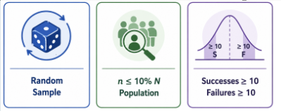
Condition 1: Randomization Condition
The data should be collected using two independent random samples.
This ensures that:
- Each sample is randomly selected from its population.
- The two samples do not influence each other.
- The observations within each sample are unbiased.
Requirement
Two independent random samples must be used.
Condition 2: 10% Condition
If sampling is performed without replacement, each sample must represent no more than 10% of its respective population.
This condition allows observations within each sample to be treated as approximately independent.
Requirement
\(\boxed{n_1\le0.10N_1 \quad\text{and}\quad n_2\le0.10N_2}\)
Where:
- \(n_1\) = Sample size from Population 1
- \(N_1\) = Size of Population 1
- \(n_2\) = Sample size from Population 2
- \(N_2\) = Size of Population 2
Randomization Condition
Two independent random samples.
10% Condition
\(n_1\le0.10N_1\)
\(n_2\le0.10N_2\)
Example 1: Conditions Satisfied
A researcher randomly selects:
- 120 students from a university with 5,000 students.
- 100 students from another university with 4,200 students.
Check the Conditions
Randomization
Both samples were selected randomly and independently.
✔ Condition satisfied.
10% Condition
\(120\le0.10(5000)=500\)
\(100\le0.10(4200)=420\)
✔ Both conditions are satisfied.
Example 2: 10% Condition Not Met
A sample of 300 people is selected from a town containing only 2,000 residents without replacement.
Check the 10% Condition
\(0.10(2000)=200\)
Since
\(300>200\)
the 10% condition is not satisfied.
The observations may no longer be approximately independent.
Summary Table
| Condition | Requirement | Purpose |
|---|---|---|
| Randomization | Two independent random samples. | Produces unbiased, independent observations. |
| 10% Condition | \(n_1\le0.10N_1\) and \(n_2\le0.10N_2\) | Ensures approximate independence when sampling without replacement. |
Important AP Exam Notes
- These conditions apply when sampling without replacement.
- The two samples must be independent random samples.
- Each sample size must be no more than 10% of its population.
- The 10% condition helps justify treating observations as approximately independent.
- Always verify these conditions before using inference procedures for two population proportions.
Common AP Exam Mistakes
| Incorrect | Correct |
|---|---|
| Using two convenience samples. | Use two independent random samples. |
| Checking the 10% condition only for one sample. | Both samples must satisfy the 10% condition. |
| Using the 10% condition for sampling with replacement. | The 10% condition is needed only when sampling without replacement. |
Example
A researcher compares the proportion of students who own a laptop at two colleges.
She randomly selects:
- 150 students from College A, which has 8,000 students.
- 180 students from College B, which has 9,500 students.
Determine whether the randomization and 10% conditions are satisfied.
▶️ Answer / Explanation
Randomization Condition:
The problem states that two independent random samples were selected.
✔ Condition satisfied.
10% Condition:
College A: \(150\le0.10(8000)=800\)
College B: \(180\le0.10(9500)=950\)
✔ Both samples satisfy the 10% condition.
Therefore, both required conditions are met.
3.9.B.2 Conditions for Experiments Involving Two Population Proportions
When data come from a randomized experiment, the conditions required for inference are different from those for random samples.
In a randomized experiment, the randomization condition is the primary requirement.
The 10% condition is not required because participants are randomly assigned to treatments rather than randomly sampled from a population.
Key Idea
If the data are collected through a randomized experiment, the treatments must be randomly assigned to the experimental units.
Random assignment helps create comparable treatment groups and supports the assumption that the groups are independent.
Randomization Condition
Experimental units must be randomly assigned to the treatment groups.
Why Is Random Assignment Important?
- Helps create treatment groups that are similar before the treatment is applied.
- Reduces the effects of confounding variables.
- Allows differences in sample proportions to be attributed to the treatments rather than pre-existing differences.
- Supports cause-and-effect conclusions when other experimental principles are also satisfied.
Random Sampling vs. Random Assignment
| Random Sampling | Random Assignment |
|---|---|
| Used in observational studies. | Used in experiments. |
| Selects individuals from a population. | Assigns selected individuals to treatment groups. |
| Supports generalizing to the population. | Supports cause-and-effect conclusions. |
Example 1
A researcher wants to compare two teaching methods.
One hundred students volunteer for the study.
The researcher randomly assigns:
- 50 students to Method A.
- 50 students to Method B.
Check the Condition
- Students were randomly assigned to treatments.
- ✔ Randomization condition is satisfied.
- The 10% condition is not required because this is a randomized experiment.
Example 2
A pharmaceutical company randomly assigns patients to receive either:
- A new medication.
- A placebo.
Because treatment assignment is random, the randomization condition is satisfied.
The experiment may proceed without checking the 10% condition.
Summary Table
| Study Type | Condition Required |
|---|---|
| Random Samples | Randomization + 10% Condition |
| Randomized Experiment | Random Assignment Only |
Important AP Exam Notes
- For randomized experiments, verify that treatments were randomly assigned.
- The 10% condition is unnecessary for randomized experiments.
- Random assignment helps create independent treatment groups.
- Random assignment supports cause-and-effect conclusions when the experiment is well designed.
- Do not confuse random sampling with random assignment.
Common AP Exam Mistakes
| Incorrect | Correct |
|---|---|
| Checking the 10% condition for every experiment. | The 10% condition is unnecessary in randomized experiments. |
| Confusing random sampling with random assignment. | Random sampling selects subjects; random assignment places subjects into treatment groups. |
| Believing random assignment guarantees a representative sample. | Random assignment supports fair treatment comparisons, not population representation. |
Example
A researcher randomly assigns 240 volunteers to receive either a new allergy medication or a placebo.
The researcher plans to compare the proportion of patients whose symptoms improve.
Explain whether the required condition for using the sampling distribution of the difference between two sample proportions is satisfied.
▶️ Answer / Explanation
This study is a randomized experiment.
Because the volunteers were randomly assigned to the treatment groups, the randomization condition is satisfied.
The 10% condition does not need to be checked because it applies only to random sampling without replacement, not to randomized experiments.
3.9.B.3 Large Counts Condition for the Sampling Distribution of the Difference Between Two Sample Proportions
To use a normal distribution to model the sampling distribution of the difference between two sample proportions, both samples must be large enough.
This is verified using the Large Counts Condition, which checks that the expected numbers of successes and failures in each sample are sufficiently large.
Key Idea
The sampling distribution of
\(\hat{p}_1-\hat{p}_2\)
can be approximated by a normal distribution if each sample has at least 10 expected successes and 10 expected failures.
Large Counts Condition
Both samples must satisfy all four conditions:
- \(\boxed{n_1p_1\ge10}\)
- \(\boxed{n_1(1-p_1)\ge10}\)
- \(\boxed{n_2p_2\ge10}\)
- \(\boxed{n_2(1-p_2)\ge10}\)
Meaning of Each Quantity
| Expression | Meaning |
|---|---|
| \(n_1p_1\) | Expected number of successes in Sample 1. |
| \(n_1(1-p_1)\) | Expected number of failures in Sample 1. |
| \(n_2p_2\) | Expected number of successes in Sample 2. |
| \(n_2(1-p_2)\) | Expected number of failures in Sample 2. |
Why Is This Condition Important?
- It ensures that each sample contains enough expected successes and failures.
- This allows the sampling distribution of the difference between sample proportions to be well approximated by a normal distribution.
- If any of the four quantities is less than 10, the normal approximation may not be appropriate.
Example 1: Condition Satisfied
A study compares two populations with:
- \(n_1=200,\; p_1=0.40\)
- \(n_2=150,\; p_2=0.70\)
Check the Conditions
\(n_1p_1=200(0.40)=80\)
\(n_1(1-p_1)=200(0.60)=120\)
\(n_2p_2=150(0.70)=105\)
\(n_2(1-p_2)=150(0.30)=45\)
All four values are at least 10.
✔ The Large Counts Condition is satisfied.
Example 2: Condition Not Satisfied
Suppose
- \(n_1=20,\; p_1=0.15\)
- \(n_2=25,\; p_2=0.60\)
Check the Conditions
\(n_1p_1=20(0.15)=3\)
Since
\(3<10\)
the Large Counts Condition is not satisfied.
The sampling distribution should not be modeled using a normal distribution.
Summary Table
| Condition | Requirement | Purpose |
|---|---|---|
| Expected Successes | \(n_1p_1\ge10,\;n_2p_2\ge10\) | Enough expected successes in both samples. |
| Expected Failures | \(n_1(1-p_1)\ge10,\;n_2(1-p_2)\ge10\) | Enough expected failures in both samples. |
Important AP Exam Notes
- All four expected counts must be at least 10.
- The Large Counts Condition justifies using a normal approximation for the sampling distribution.
- If any one of the four values is less than 10, the condition is not satisfied.
- Always check this condition before performing inference for two population proportions.
- Keep the order of the populations consistent throughout the analysis.
Common AP Exam Mistakes
| Incorrect | Correct |
|---|---|
| Checking only successes. | Check both expected successes and expected failures for each sample. |
| Checking only one sample. | Verify all four conditions for both samples. |
| Assuming the sampling distribution is always normal. | The normal approximation is appropriate only if the Large Counts Condition is satisfied. |
Example
A survey compares the proportion of students who participate in school sports at two high schools.
The population proportions are estimated as:
- \(p_1=0.55,\; n_1=120\)
- \(p_2=0.40,\; n_2=150\)
Determine whether the Large Counts Condition is satisfied.
▶️ Answer / Explanation
Sample 1
\(n_1p_1=120(0.55)=66\)
\(n_1(1-p_1)=120(0.45)=54\)
Sample 2
\(n_2p_2=150(0.40)=60\)
\(n_2(1-p_2)=150(0.60)=90\)
All four expected counts are at least 10.
✔ Therefore, the Large Counts Condition is satisfied, and a normal approximation for the sampling distribution of \(\hat{p}_1-\hat{p}_2\) is appropriate.
3.9.C.1 Interpreting the Mean, Standard Deviation, and Probabilities for the Sampling Distribution of the Difference Between Two Sample Proportions
Once the sampling distribution of the difference between two sample proportions has been established, its mean, standard deviation, and probabilities must always be interpreted in the context of the two populations being compared.
These values describe the behavior of the statistic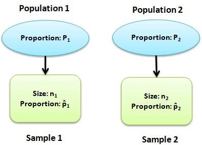
\(\hat{p}_1-\hat{p}_2\)
when many independent random samples of the same sizes are repeatedly selected from the two populations.
Interpreting the Mean
The mean of the sampling distribution is
\(\mu_{\hat{p}_1-\hat{p}_2}=p_1-p_2\)
Interpretation
Over many repeated random samples, the average difference between the sample proportions is equal to the true difference between the two population proportions.
Example
If
\(p_1=0.65\) and \(p_2=0.50\),
then
\(\mu_{\hat{p}_1-\hat{p}_2}=0.15\)
Interpretation
On average, the sample proportion from Population 1 is expected to be 0.15 (15 percentage points) higher than the sample proportion from Population 2.
Interpreting the Standard Deviation
The standard deviation measures the typical amount that
\(\hat{p}_1-\hat{p}_2\)
varies from sample to sample.
A smaller standard deviation indicates that the sample proportions are more consistent, while a larger standard deviation indicates greater sampling variability.
Example
If the standard deviation is
\(0.04\)
then the difference between the sample proportions typically varies by about 0.04 (4 percentage points) from one pair of random samples to another.
Interpreting Probabilities
Probabilities describe the likelihood that the difference between two sample proportions falls within a specified interval.
These probabilities are calculated using the sampling distribution.
Example
Suppose
\(P(\hat{p}_1-\hat{p}_2>0.10)=0.87\)
Interpretation
There is approximately an 87% probability that the difference between the sample proportions from the two random samples will be greater than 0.10.
This probability refers to the behavior of the statistic over many repeated random samples—not to the population proportions themselves.
Example
A researcher compares the proportion of students who pass an AP Statistics exam at two schools.
- School A: \(p_1=0.72\)
- School B: \(p_2=0.65\)
The sampling distribution of
\(\hat{p}_1-\hat{p}_2\)
has:
- Mean = \(0.07\)
- Standard deviation = \(0.05\)
Interpretations
- The average difference between the sample pass rates is expected to be 0.07 (7 percentage points).
- The observed differences in sample pass rates typically vary by about 0.05 (5 percentage points) from sample to sample.
- Probabilities describe how likely different sample differences are when random samples are repeatedly selected.
Important AP Exam Notes
- Interpret the mean, standard deviation, and probabilities using the context of the two populations.
- The sampling distribution describes the behavior of sample proportions, not population proportions.
- The mean is centered at the true difference, \(p_1-p_2\).
- The standard deviation measures the variability of the statistic \(\hat{p}_1-\hat{p}_2\).
- Probabilities describe what happens over many repeated random samples.
Common AP Exam Mistakes
| Incorrect | Correct |
|---|---|
| Interpreting the mean as a sample result. | The mean is the expected value of the sampling distribution. |
| Interpreting probabilities about the population proportions. | Probabilities refer to the statistic \(\hat{p}_1-\hat{p}_2\) over repeated sampling. |
| Ignoring the study context. | Always describe the results using the two specific populations in the problem. |
Example
A researcher compares the proportion of adults who exercise regularly in two cities.
The sampling distribution of \(\hat{p}_1-\hat{p}_2\) has:
- Mean = \(0.08\)
- Standard deviation = \(0.03\)
- \(P(\hat{p}_1-\hat{p}_2>0.05)=0.84\)
Interpret each value in context.
▶️ Answer / Explanation
Mean: On average, the sample proportion of adults who exercise regularly in City 1 is expected to be 0.08 (8 percentage points) higher than in City 2.
Standard Deviation: The difference between the sample proportions typically varies by about 0.03 (3 percentage points) from one pair of random samples to another.
Probability: There is approximately an 84% probability that the difference between the sample proportions from the two random samples will be greater than 0.05.