Home / AP Statistics 4.12 The Geometric  Distribution Study Notes

AP Statistics 4.12 The Geometric  Distribution Study Notes

AP Statistics 4.12 The Geometric  Distribution Study Notes- New syllabus

AP Statistics 4.12 The Geometric  Distribution Study Notes -As per latest AP Statistics Syllabus.

LEARNING OBJECTIVE

  • Probabilistic reasoning allows us to anticipate patterns in data

Key Concepts:

  • Calculating Probabilities for Geometric Random Variables
  • Parameters of a Geometric Distribution
  • Interpreting Probabilities and Parameters for a Geometric Distribution

AP Statistics -Concise Summary Notes- All Topics

Calculating Probabilities for Geometric Random Variables

Calculating Probabilities for Geometric Random Variables

A geometric random variable \( X \) counts the number of trials needed to achieve the first success in a sequence of independent trials, each with the same probability of success \( p \).

Geometric Probability Formula

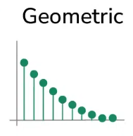
Probability that the first success occurs on the \( x \)-th trial:

  • \( P(X = x) = (1-p)^{x-1} \cdot p \)
  • Where \( x = 1, 2, 3, \dots \) and \( 0 < p \le 1 \).
  • The sum of probabilities over all possible \( x \) values is 1.

Key Points

  • Geometric random variables model the number of trials until the first success.
  • Probabilities decrease as the number of trials until the first success increases.
  • Always include context when interpreting \( P(X = x) \) (e.g., “3rd free throw”).

Example 

Suppose a basketball player has a 0.75 probability of making a free throw. Let \( X \) be the number of free throws until the first successful shot.

 Calculate \( P(X = 3) \), the probability that the first successful shot occurs on the 3rd attempt.

▶️ Answer / Explanation

Step 1: Identify the parameters: \( p = 0.75 \), \( x = 3 \).

Step 2: Use the geometric formula:

\( P(X = 3) = (1-0.75)^{3-1} \cdot 0.75 \)

Step 3: Compute:

\( P(X = 3) = (0.25)^2 \cdot 0.75 = 0.0625 \cdot 0.75 = 0.046875 \)

Answer: The probability that the first successful shot occurs on the 3rd attempt is approximately 0.047.

Parameters of a Geometric Distribution

Parameters of a Geometric Distribution

A geometric random variable \( X \) counts the number of trials until the first success. The main parameter is the probability of success \( p \) on a single trial.

Formulas for Parameters

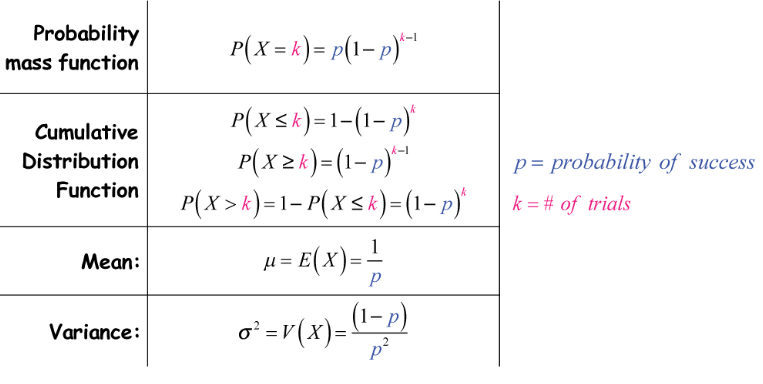
  • Mean (expected value): \( \mu_X = \dfrac{1}{p} \)
  • Variance: \( \sigma^2_X = \dfrac{1-p}{p^2} \)
  • Standard deviation: \( \sigma_X = \sqrt{\dfrac{1-p}{p^2}} \)

Interpretation

  • \( \mu_X \) gives the average number of trials needed to get the first success.
  • \( \sigma_X \) measures the typical variation in the number of trials needed.
  • All interpretations should be expressed in the context of the situation.

Example 

A basketball player has a 0.75 probability of making a free throw. Let \( X \) be the number of free throws until her first successful shot.

 Calculate the mean and standard deviation, and interpret them in context.

▶️ Answer / Explanation

Step 1: Identify parameter: \( p = 0.75 \).

Step 2: Calculate mean: \( \mu_X = \dfrac{1}{p} = \dfrac{1}{0.75} \approx 1.33 \).

Step 3: Calculate standard deviation: \( \sigma_X = \sqrt{\dfrac{1-p}{p^2}} = \sqrt{\dfrac{0.25}{0.75^2}} = \sqrt{0.4444} \approx 0.6667 \).

Step 4: Interpretation in context:

  • On average, she needs about 1.33 free throws to make her first successful shot.
  • The number of free throws until the first success typically varies by about 0.67 shots from the mean.

Interpreting Probabilities and Parameters for a Geometric Distribution

Interpreting Probabilities and Parameters for a Geometric Distribution

When working with geometric random variables, it is essential to interpret probabilities, mean, and standard deviation in the context of the problem and include appropriate units. This makes conclusions meaningful and directly related to the specific situation.

Key Concepts

  • Probability: \( P(X = x) \) represents the chance that the first success occurs on the \( x \)-th trial. Always describe what this means in context (e.g., “the probability that the player makes her first basket on the 3rd attempt”).
  • Mean (Expected Value): \( \mu_X = \dfrac{1}{p} \) tells the average number of trials needed to get the first success. Include units.
  • Standard Deviation: \( \sigma_X = \sqrt{\dfrac{1-p}{p^2}} \) indicates how much the number of trials typically varies from the mean. Include units and context.
  • All interpretations should relate directly to the population or situation described in the problem.

Note:

  • Always include units and context when interpreting probabilities and parameters.
  • Probabilities should clearly describe the event (e.g., which trial the first success occurs on).
  • Mean and standard deviation provide information about center and variability, but should be interpreted in context.

Example 

A basketball player has a 0.75 probability of making a free throw. Let \( X \) be the number of free throws until she makes her first successful shot.

 Interpret the probability that the first success occurs on the 3rd attempt, and interpret the mean and standard deviation in context.

▶️ Answer / Explanation

Step 1: Probability: \( P(X = 3) = (1-0.75)^{3-1} \cdot 0.75 = (0.25)^2 \cdot 0.75 = 0.046875 \).

Interpretation: There is approximately a 4.7% chance that the player makes her first successful free throw on the 3rd attempt.

Step 2: Mean: \( \mu_X = \dfrac{1}{0.75} \approx 1.33 \).

Interpretation: On average, the player will make her first successful shot after about 1.33 free throws.

Step 3: Standard deviation: \( \sigma_X = \sqrt{\dfrac{1-0.75}{0.75^2}} = \sqrt{0.4444} \approx 0.667 \).

Interpretation: The number of free throws until the first success typically varies by about 0.67 attempts from the mean.

Scroll to Top