Home / AP Statistics 4.2 Constructing a Confidence Interval for a Population Mean or Population Mean Difference Study Notes

AP Statistics 4.2 Constructing a Confidence Interval for a Population Mean or Population Mean Difference Study Notes - New Syllabus

AP Statistics 4.2 One-Sample t-Intervals for a Population Mean Study Notes – New Syllabus

AP Statistics 4.2 One-Sample t-Intervals for a Population Mean Study Notes – As per latest AP Statistics Syllabus.

LEARNING OBJECTIVES

  • 4.2.A Describe t-distributions.
  • 4.2.B Identify an appropriate confidence interval procedure including the parameter for a population mean or population mean difference.
  • 4.2.C Justify the appropriateness of constructing a confidence interval for a population mean or population mean difference by verifying conditions.
  • 4.2.D Calculate an appropriate confidence interval for a population mean or population mean difference.
  • 4.2.E Calculate the standard error and margin of error for a sample size or a one-sample t-interval.

ESSENTIAL KNOWLEDGE:

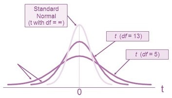
  • 4.2.A.1 t-distributions, also called Student’s t-distributions, form a family of symmetric, bell-shaped, standardized distributions with wider tails than that of the standard normal distribution. Specific t-distributions are identified using a parameter known as the number of degrees of freedom (df), which is based on the sample size(s). When the degrees of freedom are small, the t-distribution has a much narrower peak and fatter tails than a normal distribution. As the degrees of freedom increase, the t-distribution more closely resembles the standard normal distribution (mean \( \mu=0 \) and standard deviation \( \sigma=1 \)).
  • 4.2.A.2 t-distributions are used for finding critical values and test statistics for inferences about a population mean, \( \mu \), when the population standard deviation, \( \sigma \), is unknown and the sample standard deviation, \( s \), must be used instead.
  • 4.2.B.1 The appropriate confidence interval procedure for estimating the population mean of a quantitative variable for one sample is a one-sample t-interval for a population mean. (The population standard deviation, \( \sigma \), is not typically known for distributions for quantitative variables.)
  • 4.2.B.2 For a matched pairs design with two dependent samples, the appropriate analysis calculates differences between pairs of values to produce one sample of differences. The confidence interval procedure for the matched pairs design is a one-sample t-interval for a population mean difference.
  • 4.2.B.3 The parameter for a confidence interval for a population mean or population mean difference should reference the population mean or population mean difference and the response variable, in context. For the population mean difference, it is important to state the order of subtraction for the difference.
  • 4.2.C.1 A one-sample t-interval for a population mean or population mean difference requires that three conditions be met:
    • 4.2.C.1.i The randomization condition—the data should be collected using a random sample or a randomized experiment.
    • 4.2.C.1.ii The 10% condition—when sampling without replacement, the population size must be at least 10 times larger than the sample size (\( n \le 10\%N \)), where \( N \) is the size of the population and \( n \) is the sample size.
    • 4.2.C.1.iii The sample data condition—it is indicated the population distribution is approximately normal, or \( n \ge 30 \), or if \( n < 30 \), the sample data distribution should be free from strong skewness and outliers. For matched pairs, the number of differences should be greater than or equal to 30. If the number of differences is less than 30, the sample of differences should be free from strong skewness and outliers.
  • 4.2.D.1 A point estimate for a population mean is the sample mean, \( \bar{x} \), or \( \bar{x}_d \) for the sample mean difference.
  • 4.2.D.2 To estimate the population mean for one sample or the population mean difference between values in matched pairs, when the population standard deviation is unknown, the confidence interval is

    \( \bar{x}\pm t^*\left(\dfrac{s}{\sqrt{n}}\right) \)

    where \( t^* \) is the critical value for the central \( C\% \) of a t-distribution with degrees of freedom \( n-1 \).
  • 4.2.E.1 The standard error (SE) for a sample mean is given by

    \( SE_{\bar{x}}=\dfrac{s}{\sqrt{n}} \)
  • 4.2.E.2 For a one-sample t-interval for a population mean, the margin of error is the critical value (\( t^* \)) times the standard error (SE), which equals

    \( \left(t^*\right)\left(\dfrac{s}{\sqrt{n}}\right) \)

AP Statistics – Concise Summary Notes – All Topics


4.2.A.1 t-Distributions (Student’s t-Distributions)

When making inferences about a population mean, statisticians often use a t-distribution instead of the standard normal distribution.

A t-distribution, also called a Student’s t-distribution, is a family of probability distributions that are symmetric, bell-shaped, and centered at 0.

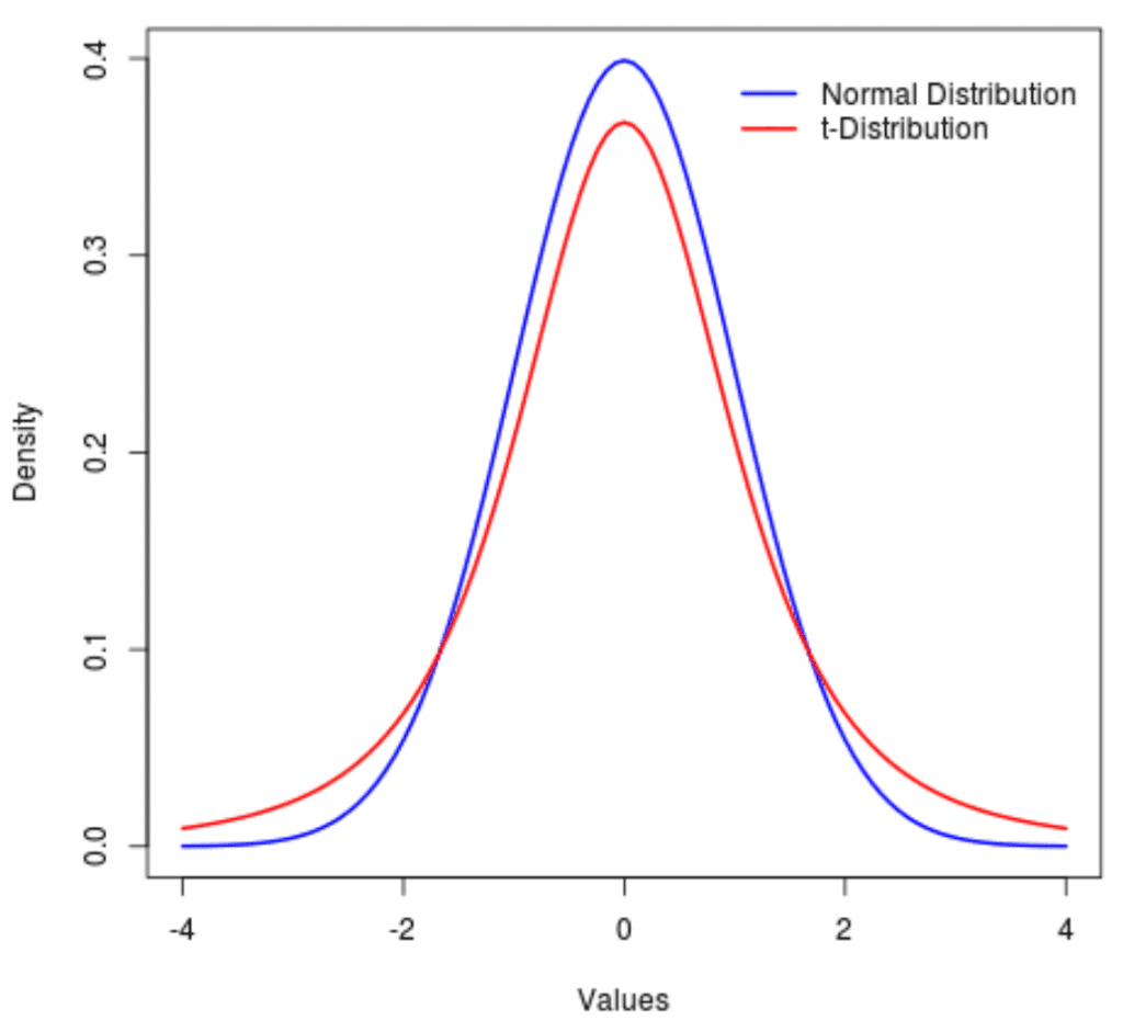
Unlike the standard normal distribution, a t-distribution has wider (heavier) tails. These heavier tails account for the additional uncertainty that occurs when the population standard deviation (\( \sigma \)) is unknown and must be estimated using the sample standard deviation.

Each t-distribution is identified by its degrees of freedom (df), which depend on the sample size. 
For a one-sample t-distribution, the degrees of freedom are calculated as

\( \mathrm{df}=n-1 \)

Where:

  • \(n\) = Sample size
  • \(\mathrm{df}\) = Degrees of freedom

When the degrees of freedom are small, the t-distribution has a lower peak and fatter tails than the standard normal distribution.

As the degrees of freedom increase, the t-distribution becomes more similar to the standard normal distribution.

For very large degrees of freedom, the t-distribution is nearly identical to the standard normal distribution, which has

  • \( \mu=0 \)
  • \( \sigma=1 \)
Characteristict-Distribution
ShapeSymmetric and bell-shaped
Center0
SpreadDepends on the degrees of freedom
TailsWider (heavier) than the standard normal distribution
ParameterDegrees of freedom (\(\mathrm{df}\))

Comparing the t-Distribution and the Standard Normal Distribution
Standard Normal Distributiont-Distribution
Mean \(=0\), Standard Deviation \(=1\)Centered at 0 with spread determined by the degrees of freedom
One unique distributionA family of distributions, each with a different degrees of freedom
Thinner tailsHeavier (wider) tails
Used when \( \sigma \) is knownUsually used when \( \sigma \) is unknown

4.2.A.2 When to Use a t-Distribution

A t-distribution is used when making statistical inferences about a population mean (\(\mu\)) and the population standard deviation (\(\sigma\)) is unknown.

Since the population standard deviation is usually unknown, it is estimated using the sample standard deviation (\(s\)).

Therefore, the t-distribution is commonly used when constructing confidence intervals and performing hypothesis tests for a population mean.

Known InformationDistribution Used
Population standard deviation (\(\sigma\)) is knownStandard Normal (z)
Population standard deviation (\(\sigma\)) is unknown and sample standard deviation (\(s\)) is usedt-Distribution

Important AP Exam Notes

  • A t-distribution is a family of distributions identified by the degrees of freedom.
  • For one-sample procedures, the degrees of freedom are calculated using \( \mathrm{df}=n-1 \).
  • Smaller degrees of freedom produce fatter tails and a lower peak.
  • As the degrees of freedom increase, the t-distribution approaches the standard normal distribution.
  • Use the t-distribution whenever the population standard deviation is unknown and the sample standard deviation is used instead.

Example

A random sample of 16 students is selected to estimate the average number of hours spent studying each week.

The population standard deviation is unknown, so the sample standard deviation is used.

Determine:

  1. The appropriate distribution to use.
  2. The degrees of freedom.
▶️ Answer / Explanation

Step 1: Determine the appropriate distribution.

Because the population standard deviation is unknown, a t-distribution should be used.

Step 2: Calculate the degrees of freedom.

\( \mathrm{df}=n-1 \)

\( =16-1 \)

\( =15 \)

Answer:

  • Distribution: t-distribution
  • Degrees of freedom: \(15\)

4.2.B.1 One-Sample t-Interval for a Population Mean

A one-sample t-interval is used to estimate the value of a population mean (\(\mu\)) when data are collected from a single random sample of a quantitative variable.

In most real-world situations, the population standard deviation (\(\sigma\)) is unknown. Therefore, the sample standard deviation (\(s\)) is used to estimate the population standard deviation.

Because \( \sigma \) is unknown, the confidence interval is based on the t-distribution rather than the standard normal (z) distribution.

When to Use a One-Sample t-Interval

  • The data consist of one random sample.
  • The response variable is quantitative.
  • The goal is to estimate a population mean.
  • The population standard deviation (\(\sigma\)) is unknown.

Parameter of Interest

\( \mu \) = the true population mean of the response variable.

CharacteristicOne-Sample t-Interval
Data TypeQuantitative
Number of SamplesOne random sample
ParameterPopulation mean (\(\mu\))
Population Standard DeviationUnknown
Distribution Usedt-distribution

How to Identify This Procedure on the AP Exam

  • Look for a single sample of quantitative data.
  • The question asks you to estimate an average (mean).
  • The population standard deviation is not given (or is stated to be unknown).
  • If all of these conditions are true, the correct procedure is a one-sample t-interval for a population mean.

Important AP Exam Notes

  • Do not use a z-interval unless the population standard deviation (\(\sigma\)) is known.
  • The parameter always refers to the population mean, not the sample mean.
  • Always identify the parameter in the context of the problem.
  • State both the procedure and the parameter when answering AP Statistics free-response questions.

 Example

A school administrator wants to estimate the average number of hours students sleep each night.

A random sample of 40 students is selected, and each student reports the number of hours they sleep on a typical school night.

The population standard deviation is unknown.

Identify the appropriate confidence interval procedure and state the parameter of interest.

▶️ Answer / Explanation

Procedure:

Because the data come from one random sample of a quantitative variable, and the population standard deviation is unknown, the appropriate procedure is a

One-sample t-interval for a population mean.

Parameter:

\( \mu \) = the true mean number of hours that all students at the school sleep on a typical school night.

Why not a z-interval?

A z-interval cannot be used because the population standard deviation (\(\sigma\)) is unknown. Therefore, the sample standard deviation (\(s\)) must be used, requiring the t-distribution.

4.2.B.2 One-Sample t-Interval for a Population Mean Difference (Matched Pairs)

Some studies compare two related measurements collected from the same individual or from matched individuals.

This type of study is called a matched pairs design because each observation in one sample is naturally paired with a corresponding observation in the other sample.

Instead of analyzing the two samples separately, the difference between each pair of observations is calculated.

These differences form one sample of quantitative data.

The appropriate confidence interval procedure is then a one-sample t-interval for a population mean difference.

Because the population standard deviation of the differences is unknown, the sample standard deviation of the differences is used, so the t-distribution is required.

When to Use a Matched Pairs t-Interval

  • The data consist of matched pairs or repeated measurements.
  • The observations are dependent, not independent.
  • The difference between each pair is calculated.
  • The goal is to estimate the population mean difference.
  • The population standard deviation of the differences is unknown.

Parameter of Interest

\( \mu_d \) = the true population mean difference.

It is important to clearly define the difference, such as

Difference = After − Before

or

Difference = Treatment − Control

The order of subtraction must remain the same throughout the analysis.

CharacteristicMatched Pairs t-Interval
Data TypeQuantitative
Study DesignMatched pairs (dependent observations)
Data AnalyzedDifferences between each pair
Parameter\( \mu_d \)
Distribution Usedt-distribution

How to Identify This Procedure on the AP Exam

  • Look for words such as before and after, pre-test and post-test, same subjects, matched pairs, or paired observations.
  • If each individual contributes two related measurements, calculate the differences first.
  • Treat the differences as a single sample.
  • Use a one-sample t-interval for a population mean difference.

Important AP Exam Notes

  • Matched pairs data are dependent, not independent.
  • Always calculate the differences first.
  • The parameter is the population mean difference, not two separate population means.
  • Always state the order of subtraction when defining the differences.
  • Because the population standard deviation is unknown, use the t-distribution.

 Example

A fitness trainer wants to determine whether a new workout program changes the average number of push-ups participants can complete.

Twenty participants complete a push-up test before starting the program and again after six weeks of training.

Identify the appropriate confidence interval procedure and state the parameter of interest.

▶️ Answer / Explanation

Step 1: Identify the study design.

The same participants are measured twice (before and after training), so the data are matched pairs.

Step 2: Determine the procedure.

Calculate the difference for each participant:

Difference = After − Before

Then use a

One-sample t-interval for a population mean difference.

Parameter:

\( \mu_d \) = the true mean difference in the number of push-ups completed (After − Before) for all participants who follow the workout program.

4.2.B.3 Identifying the Parameter for a Population Mean or Population Mean Difference

When constructing a confidence interval, it is important to clearly identify the parameter of interest.

A parameter is a numerical characteristic of a population, not a sample.

The parameter should always be written in the context of the problem and should describe the population being studied.

The appropriate parameter depends on whether the study involves one sample or matched pairs.


Parameter for One-Sample Procedures

When estimating a single population mean, the parameter is

\( \mu \)

where

\( \mu \) = the true population mean of the response variable.

Always describe the response variable and the population in context.

Example Parameter Statement

\( \mu \) = the true mean number of hours that all students at the school sleep each night.


Parameter for Matched Pairs Procedures

When using a matched pairs design, the parameter is the population mean difference.

This parameter is written as

\( \mu_d \)

where

\( \mu_d \) = the true population mean difference.

Before defining the parameter, you must clearly specify the order of subtraction.

For example, if the differences are calculated as

Difference = After − Before

then the parameter should be written as

\( \mu_d \) = the true mean value of (After − Before) for the population.

If the order of subtraction is reversed, the interpretation also changes.

Study DesignParameterContext
One Sample\( \mu \)True population mean of the response variable.
Matched Pairs\( \mu_d \)True population mean difference, with the order of subtraction clearly stated.

Important AP Exam Notes

  • The parameter always refers to the population, never the sample.
  • Include the response variable and the population when defining the parameter.
  • For matched pairs, always define the difference before writing the parameter.
  • The order of subtraction (such as After − Before or Treatment − Control) must remain consistent throughout the analysis.
  • Failure to define the order of subtraction may result in an incorrect interpretation on the AP Exam.

Example

A researcher wants to determine whether a new tutoring program improves students’ mathematics test scores.

Each student takes a mathematics test before participating in the tutoring program and another test after completing the program.

Identify the parameter of interest.

▶️ Answer / Explanation

Step 1: Identify the study design.

The same students are tested twice, so this is a matched pairs design.

Step 2: Define the difference.

Difference = After − Before

Step 3: State the parameter.

\( \mu_d \) = the true mean difference in mathematics test scores (After − Before) for all students who participate in the tutoring program.

Notice that the order of subtraction, After − Before, is clearly stated in the parameter.

4.2.C.1 Conditions for Constructing a One-Sample t-Interval

Before constructing a one-sample t-interval for a population mean or a population mean difference, statisticians must verify that the required conditions are satisfied.

These conditions ensure that the resulting confidence interval provides a valid estimate of the population parameter.

A one-sample t-interval requires the following three conditions:

  • Randomization Condition
  • 10% Condition
  • Sample Data Condition

4.2.C.1.i Randomization Condition

The data should come from a random sample or a randomized experiment.

Randomization helps reduce bias and allows the sample to be representative of the population.

How to Verify

  • The problem states that a simple random sample (SRS) was selected.
  • The problem states that the sample was randomly selected.
  • The experiment used random assignment to treatments.

4.2.C.1.ii 10% Condition

When sampling is done without replacement, the sample should be less than 10% of the population.

This condition allows the observations to be treated as approximately independent.

Formula

\( N \ge 10n \)

or equivalently

\( n \le 0.10N \)

Where:

  • \(N\) = Population size
  • \(n\) = Sample size

4.2.C.1.iii Sample Data Condition

The t-procedures require that the sampling distribution of the sample mean (or sample mean difference) be approximately normal.

This condition can be satisfied in several ways.

SituationCondition Satisfied?
Population distribution is approximately normal.✔ Yes
Sample size \( n \ge 30 \).✔ Yes (Central Limit Theorem)
Sample size \( n < 30 \), but the sample data show no strong skewness or outliers.✔ Yes
Sample size \( n < 30 \) with strong skewness or outliers.✘ No

Matched Pairs Studies

For matched pairs, the observations are first converted into a single sample of differences.

  • If the number of differences is \( n \ge 30 \), the Sample Data Condition is satisfied.
  • If \( n < 30 \), the distribution of the differences should be free from strong skewness and outliers.

Summary of the Conditions

ConditionRequirement
RandomizationRandom sample or randomized experiment.
10% Condition\( N \ge 10n \) when sampling without replacement.
Sample Data ConditionPopulation is approximately normal, or \( n \ge 30 \), or if \( n < 30 \), the sample data (or differences) are free from strong skewness and outliers.

Important AP Exam Notes

  • Always verify all three conditions before constructing a one-sample t-interval.
  • When \( n < 30 \), examine the sample data (or differences for matched pairs) for strong skewness and outliers.
  • The 10% Condition applies only when sampling is performed without replacement.
  • When justifying conditions on the AP Exam, explicitly state whether each condition is satisfied and explain why.

 Example

A researcher randomly selects 25 students from a school of 800 students to estimate the average number of hours they study each week.

The distribution of study times is approximately symmetric with no outliers.

Determine whether it is appropriate to construct a one-sample t-interval.

▶️ Answer / Explanation

Step 1: Randomization Condition

The problem states that a random sample of students was selected.

✔ The Randomization Condition is satisfied.

Step 2: 10% Condition

Population size:

\( N=800 \)

Sample size:

\( n=25 \)

Check the condition:

\( 10n=250 \)

Since

\( 800 \ge 250 \)

✔ The 10% Condition is satisfied.

Step 3: Sample Data Condition

The sample size is less than 30, but the distribution is approximately symmetric with no outliers.

✔ The Sample Data Condition is satisfied.

Conclusion:

Because all three conditions are satisfied, it is appropriate to construct a one-sample t-interval for a population mean.

4.2.D.1 Point Estimate for a Population Mean

Before constructing a confidence interval, statisticians first calculate a point estimate for the population parameter.
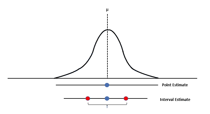
A point estimate is a single numerical value obtained from a sample that is used to estimate an unknown population parameter.

For estimating a population mean, the point estimate is the sample mean.

Point Estimate for One Sample

\( \bar{x} \)

where

  • \( \bar{x} \) = Sample mean
  • \( \mu \) = Population mean (unknown parameter)

Thus, the sample mean \( \bar{x} \) is the best point estimate of the unknown population mean \( \mu \).

Point Estimate for Matched Pairs

For a matched pairs design, the difference between each pair of observations is calculated first.

The point estimate for the population mean difference is the sample mean of the differences.

\( \bar{x}_d \)

where

  • \( \bar{x}_d \) = Sample mean of the differences
  • \( \mu_d \) = Population mean difference
SituationPoint EstimatePopulation Parameter
One Sample\( \bar{x} \)\( \mu \)
Matched Pairs\( \bar{x}_d \)\( \mu_d \)

Important AP Exam Notes

  • A point estimate is a single value used to estimate an unknown population parameter.
  • For one-sample procedures, the point estimate of \( \mu \) is the sample mean \( \bar{x} \).
  • For matched pairs, the point estimate of \( \mu_d \) is the sample mean of the differences \( \bar{x}_d \).
  • A point estimate provides only one estimate and does not describe the uncertainty of the estimate. A confidence interval is used for that purpose.

Example

A random sample of 36 students is selected to estimate the average number of hours they study each week.

The sample mean study time is

\( \bar{x}=8.4 \) hours.

Identify the point estimate for the population mean.

▶️ Answer / Explanation

The point estimate for the population mean is the sample mean.

\( \bar{x}=8.4 \) hours.

Therefore, the best point estimate of the true average number of hours studied per week by all students is 8.4 hours.

4.2.D.2 Confidence Interval for a Population Mean

A confidence interval provides a range of plausible values for an unknown population mean.

When the population standard deviation (\( \sigma \)) is unknown, the interval is constructed using the t-distribution and the sample standard deviation (\( s \)).

Confidence Interval Formula

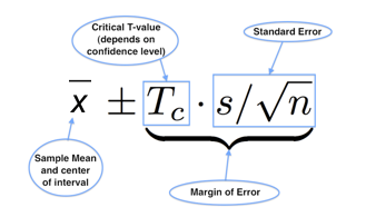
\( \bar{x}\pm t^{*}\left(\dfrac{s}{\sqrt{n}}\right) \)

Where:

  • \( \bar{x} \) = Sample mean (point estimate)
  • \( t^{*} \) = Critical value from the t-distribution with \( n-1 \) degrees of freedom
  • \( s \) = Sample standard deviation
  • \( n \) = Sample size
  • \( \dfrac{s}{\sqrt{n}} \) = Standard error of the sample mean

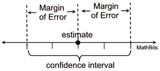
The confidence interval is centered at the sample mean and extends by a margin of error on each side.

Margin of Error

\( \text{Margin of Error}=t^{*}\left(\dfrac{s}{\sqrt{n}}\right) \)

ComponentMeaning
\( \bar{x} \)Point estimate of the population mean.
\( t^{*} \)Critical value based on the confidence level and degrees of freedom.
\( \dfrac{s}{\sqrt{n}} \)Standard error of the sample mean.
Margin of ErrorMaximum expected difference between the sample mean and the population mean.

Important AP Exam Notes

  • Use a t-interval whenever the population standard deviation is unknown. 
  • The degrees of freedom are

\( df=n-1 \)

  • The confidence interval is always written as

Point Estimate ± Margin of Error

  • The sample mean is always the center of the confidence interval.

Example

A random sample of 25 students has \( \bar{x}=72 \) \( s=10 \)

A 95% confidence interval is to be constructed.

The critical value is \( t^{*}=2.064 \)

Construct the confidence interval.

▶️ Answer / Explanation

Step 1: Calculate the standard error.

\( \dfrac{s}{\sqrt{n}}=\dfrac{10}{\sqrt{25}}=2 \)

Step 2: Calculate the margin of error.

\( ME=2.064(2)=4.128 \)

Step 3: Construct the interval.

\( 72\pm4.128 \)

\( (67.872,\;76.128) \)

The 95% confidence interval for the population mean is

\((67.872,\;76.128)\)

4.2.E.1 Standard Error for a One-Sample t-Interval

When estimating a population mean using a one-sample t-interval, the variability of the sample mean is measured by the standard error (SE).

The standard error estimates how much the sample mean is expected to vary from one random sample to another.

Since the population standard deviation (\( \sigma \)) is unknown, the sample standard deviation (\( s \)) is used to calculate the standard error.

Formula

\( SE_{\bar{x}}=\dfrac{s}{\sqrt{n}} \)

Where:

  • \( SE_{\bar{x}} \) = Standard error of the sample mean
  • \( s \) = Sample standard deviation
  • \( n \) = Sample size

The standard error measures the typical distance between the sample mean and the population mean.

As the sample size increases, the standard error decreases because larger samples produce more precise estimates of the population mean.

QuantityFormulaInterpretation
Standard Error\( \dfrac{s}{\sqrt{n}} \)Measures the variability of sample means from sample to sample.

Important AP Exam Notes

  • Standard error is calculated using the sample standard deviation (\(s\)), not the population standard deviation.
  • The standard error is always positive.
  • As the sample size increases, the standard error decreases.
  • A smaller standard error results in a more precise estimate of the population mean.

 Example

A random sample of 36 students has a sample standard deviation of

\( s=12 \)

Calculate the standard error of the sample mean.

▶️ Answer / Explanation

Step 1: Write the formula.

\( SE_{\bar{x}}=\dfrac{s}{\sqrt{n}} \)

Step 2: Substitute the given values.

\( SE_{\bar{x}}=\dfrac{12}{\sqrt{36}} \)

Step 3: Simplify.

\( SE_{\bar{x}}=\dfrac{12}{6}=2 \)

Answer:

The standard error is \(2\).

4.2.E.2 Margin of Error for a One-Sample t-Interval

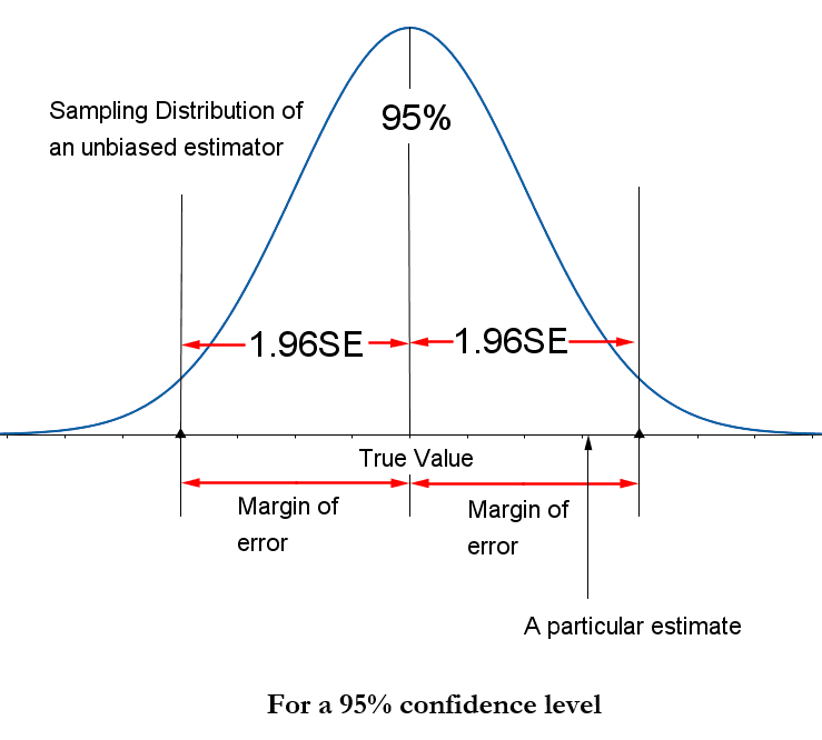
The margin of error (ME) measures the maximum expected difference between the sample mean and the true population mean for a given confidence level.

For a one-sample t-interval, the margin of error is equal to the critical value multiplied by the standard error.
Formula

\( ME=t^{*}\left(\dfrac{s}{\sqrt{n}}\right) \)

Where:

  • \( ME \) = Margin of error
  • \( t^{*} \) = Critical value from the t-distribution
  • \( s \) = Sample standard deviation
  • \( n \) = Sample size

A larger confidence level produces a larger critical value, which increases the margin of error.

Similarly, increasing the sample size decreases the standard error, resulting in a smaller margin of error.

QuantityFormulaPurpose
Margin of Error\( t^{*}\left(\dfrac{s}{\sqrt{n}}\right) \)Determines how far the confidence interval extends from the sample mean.

Important AP Exam Notes

  • The margin of error is always positive.
  • A larger sample size produces a smaller margin of error.
  • A higher confidence level produces a larger margin of error.
  • The confidence interval is always written as

Point Estimate ± Margin of Error

Example

A random sample of 25 students has \( s=10 \)

The critical value for a 95% confidence interval is \( t^{*}=2.064 \)

Calculate the margin of error.

▶️ Answer / Explanation

Step 1: Calculate the standard error.

\( SE=\dfrac{10}{\sqrt{25}}=\dfrac{10}{5}=2 \)

Step 2: Calculate the margin of error.

\( ME=2.064(2)=4.128 \)

Answer:

The margin of error is \(4.128\).

Scroll to Top