Home / AP Statistics 4.3 Introduction  to Probability Study Notes

AP Statistics 4.3 Introduction  to Probability Study Notes

AP Statistics 4.3 Introduction  to Probability Study Notes- New syllabus

AP Statistics 4.3 Introduction  to Probability Study Notes -As per latest AP Statistics Syllabus.

LEARNING OBJECTIVE

  • The likelihood of a random event can be quantified.

Key Concepts:

  • Introduction to Probability
  • Interpret Probabilities for Events

AP Statistics -Concise Summary Notes- All Topics

Introduction to Probability

Introduction to Probability

Probability is the study of randomness. It provides a mathematical framework for describing uncertain events and predicting long-term outcomes. In AP Statistics, probability connects random processes to statistical inference.

Key Concepts of Probability 

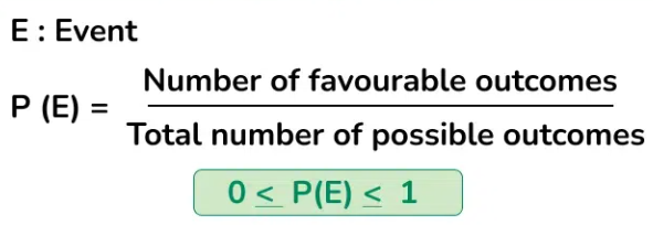
  • Randomness: Outcomes are uncertain in the short run but follow predictable patterns in the long run.
  • Experiment: A repeatable process that produces outcomes (e.g., rolling a die, flipping a coin).
  • Outcome: A possible result of a chance experiment (e.g., rolling a “4”).
  • Sample Space (S): The set of all possible outcomes (e.g., S = {1,2,3,4,5,6} for a die roll).
  • Event: A subset of the sample space (e.g., rolling an even number = {2,4,6}).

Rules of Probability

  • Probabilities are always between 0 and 1 (0 ≤ P(A) ≤ 1).
  • The probability of the entire sample space is 1: P(S) = 1.
  • The probability of an event not happening: P(Not A) = 1 − P(A).
  • If two events are mutually exclusive (cannot occur together), then P(A or B) = P(A) + P(B).
  • In general: P(A or B) = P(A) + P(B) − P(A and B).

Types of Probability

  • Theoretical Probability: Based on mathematical reasoning and equally likely outcomes (e.g., P(rolling a 3) = 1/6).
  • Experimental Probability: Based on actual trials and outcomes (e.g., rolling a die 100 times and getting 18 threes → 18/100 = 0.18).
  • Subjective Probability: Based on personal judgment or experience, not precise calculations (e.g., “I think there’s a 70% chance it will rain tomorrow”).

Comparison Table

ConceptDefinitionExample
Sample Space (S)All possible outcomes of a chance experimentRolling a die: {1,2,3,4,5,6}
EventSubset of the sample spaceRolling an even number: {2,4,6}
Theoretical ProbabilityBased on equally likely outcomesP(rolling a 3) = 1/6
Experimental ProbabilityBased on observed outcomes from trials18 threes in 100 rolls → 0.18
Subjective ProbabilityBased on personal judgment70% chance of rain

Example 

What is the probability of rolling a number greater than 4 on a fair six-sided die?

▶️ Answer / Explanation

Step 1: Sample space = {1,2,3,4,5,6}.

Step 2: Favorable outcomes = {5,6} → 2 outcomes.

Step 3: Probability = 2/6 = 1/3.

Conclusion: P(number > 4) = 1/3.

Example 

A spinner has 4 equal sections labeled A, B, C, and D. What is the probability of not landing on C?

▶️ Answer / Explanation

Step 1: Sample space = {A, B, C, D}.

Step 2: P(C) = 1/4.

Step 3: P(Not C) = 1 − 1/4 = 3/4.

Conclusion: Probability = 0.75.

Example 

In 50 rolls of a die, a student gets “2” exactly 11 times. What is the experimental probability of rolling a 2?

▶️ Answer / Explanation

Step 1: Number of favorable outcomes = 11.

Step 2: Total trials = 50.

Step 3: Experimental probability = 11/50 = 0.22.

Conclusion: P(rolling a 2) ≈ 0.22.

Interpret Probabilities for Events

Interpret Probabilities for Events

Probabilities of events in repeatable situations can be interpreted as the relative frequency with which the event occurs in the long run.

  • Probability describes the proportion of times an outcome would occur if a random process were repeated many times under identical conditions.
  • It does not predict what will happen in one trial but what we expect over many trials.
  • As the number of trials increases, the relative frequency (observed probability) approaches the true theoretical probability.

Formal Definition:

If an event \( A \) occurs \( k \) times out of \( n \) trials, then the probability is approximated by:

\( P(A) \approx \dfrac{k}{n} \)

As \( n \to \infty \), the relative frequency \( \dfrac{k}{n} \) approaches the true probability \( P(A) \).

Interpretation in Context:

  • \( P(A) = 0.2 \): In the long run, the event \( A \) occurs about 20% of the time.
  • \( P(A) = 0.5 \): The event occurs about half the time in many repetitions.
  • \( P(A) = 0.9 \): The event occurs almost every time (very likely).
  • \( P(A) = 0.01 \): The event is very rare — it occurs about once in 100 trials on average.

Example :

A factory produces batteries, and the probability that a battery is defective is \( P(\text{defective}) = 0.05 \).

Interpret this probability.

▶️ Answer / Explanation
  • If the production process continues under the same conditions for many batteries, about 5% of them will be defective in the long run.
  • This means that in a batch of 1,000 batteries, we expect roughly \( 0.05 \times 1000 = 50 \) defective batteries.
  • The probability does not guarantee exactly 5% in any one batch, but rather describes the long-run proportion over many batches.

Conclusion: Probability describes a long-run relative frequency, not a single short-term prediction.

Example :

A fair coin is flipped repeatedly. The theoretical probability of getting heads is \( P(\text{Heads}) = 0.5 \).

After 10 flips, the result was: 7 heads and 3 tails.

Question: Does this result contradict the probability model?

▶️ Answer / Explanation
  • No — it does not contradict the model.
  • In the short run, random variation can cause the proportion of heads to differ from 0.5.
  • However, if the coin were flipped many more times (e.g., 1,000 or 10,000 flips), the relative frequency of heads would get closer to 0.5.
  • This illustrates the Law of Large Numbers: the observed probability approaches the true probability as the number of trials increases.

Conclusion: \( P(\text{Heads}) = 0.5 \) means that in the long run, about half of all flips result in heads.

Scroll to Top