Represent the Probability Distribution for a Discrete Random Variable
A probability distribution for a discrete random variable describes how likely each possible value of the variable is. It can be represented using tables, graphs, or functions.
Random Variable: A random variable is a numerical outcome of a random process. We usually denote it with a capital letter (e.g., \(X\)).
Discrete Random Variable: A variable that can only take on countable values (e.g., 0, 1, 2, 3…). Examples: number of heads in coin tosses, number of goals in a game.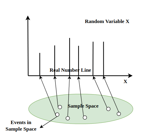
Probability Distribution:
A listing or function showing each possible value of \(X\) and the probability \(P(X = x)\) associated with it.
Validity Conditions:
- Each probability must satisfy \( 0 \leq P(X = x) \leq 1 \).
- The probabilities must sum to 1: \( \sum P(X = x) = 1 \).
Cumulative Probability Distribution (CDF):
A function or table showing \( P(X \leq x) \), i.e., the probability the random variable is less than or equal to each possible value.
Ways to Represent a Discrete Probability Distribution:
- Table: List all possible values with their probabilities.
- Graph: Bar graph of probabilities (vertical axis = probability, horizontal axis = values of \(X\)).
- Function: Define a rule for \( P(X = x) \). Example: For a fair die, \( P(X = x) = \dfrac{1}{6} \) for \( x = 1, 2, 3, 4, 5, 6 \).
Example
A fair coin is flipped twice. Let \(X\) = number of heads. Construct the probability distribution.
▶️ Answer / Explanation
Step 1: Possible outcomes: HH, HT, TH, TT.
Step 2: Possible values of \(X\): 0, 1, 2.
Step 3: Compute probabilities:
- \(P(X = 0) = \dfrac{1}{4}\) (TT only)
- \(P(X = 1) = \dfrac{2}{4} = \dfrac{1}{2}\) (HT, TH)
- \(P(X = 2) = \dfrac{1}{4}\) (HH)
| x (number of heads) | P(X = x) |
|---|---|
| 0 | 1/4 |
| 1 | 1/2 |
| 2 | 1/4 |
Example
A fair coin is flipped twice. Let \(X\) = number of heads. Construct and interpret the cumulative probability distribution of \(X\).
▶️ Answer / Explanation
Step 1: Possible values of \(X\): 0, 1, 2.
Step 2: Find cumulative probabilities:
- \(P(X \leq 0) = P(X = 0) = \dfrac{1}{4}\)
- \(P(X \leq 1) = P(X = 0) + P(X = 1) = \dfrac{1}{4} + \dfrac{1}{2} = \dfrac{3}{4}\)
- \(P(X \leq 2) = P(X = 0) + P(X = 1) + P(X = 2) = 1\)
| x | P(X ≤ x) |
|---|---|
| 0 | 0.25 |
| 1 | 0.75 |
| 2 | 1.00 |
Interpretation: The CDF shows cumulative probabilities. For example, \(P(X \leq 1) = 0.75\) means there is a 75% chance of getting at most 1 head in two flips.
Interpret a Probability Distribution
Interpreting a probability distribution means describing what the distribution tells us about the possible values of a random variable, their likelihoods, and what conclusions we can draw about the population.
Shape: Describes the overall pattern of the distribution.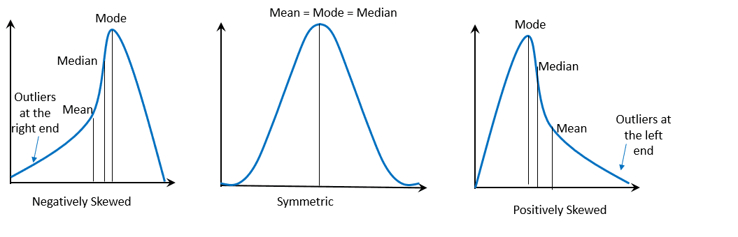
- Symmetric, skewed left, or skewed right.
- Can be uniform (all values equally likely), bell-shaped, or irregular.
- Shape helps identify patterns in the data (e.g., most values centered or extreme values more common).
Center: The “typical” or “expected” value of the random variable.
- Measured using the mean of the distribution: \( \mu = \sum x \cdot P(X = x) \).
- The mean represents the long-run average value if the random process is repeated many times.
Spread: Describes the variability of the distribution.
- Measured using the variance: \( \sigma^2 = \sum (x – \mu)^2 \cdot P(X = x) \).
- The standard deviation \( \sigma \) is the square root of variance and shows the average distance from the mean.
Probability Statements: Allows calculation of how likely certain outcomes are.
- Example: \( P(X \leq k) \) or \( P(X \geq k) \).
- These probabilities provide insight into the population’s behavior.
Example
A random variable \(X\) = number of goals scored by a soccer team in a match has the following probability distribution:
| x (Goals) | P(X = x) |
|---|---|
| 0 | 0.10 |
| 1 | 0.30 |
| 2 | 0.40 |
| 3 | 0.15 |
| 4 | 0.05 |
▶️ Answer / Explanation
- Shape: The distribution is roughly symmetric and unimodal, centered around 2 goals.
- Center: The expected value (mean) is \(\mu = 0(0.10) + 1(0.30) + 2(0.40) + 3(0.15) + 4(0.05) = 1.75\).
- Spread: Most of the probability mass lies between 1 and 3 goals. Variance and standard deviation can be calculated for precision.
- Probability Statements:
- \(P(X \geq 2) = 0.40 + 0.15 + 0.05 = 0.60\). → There is a 60% chance the team scores 2 or more goals.
- \(P(X = 0) = 0.10\). → The team has a 10% chance of not scoring any goals.