AP Statistics 4.8 Mean and Standard Deviation of Random Variables Study Notes
AP Statistics 4.8 Mean and Standard Deviation of Random Variables Study Notes- New syllabus
AP Statistics 4.8 Mean and Standard Deviation of Random Variables Study Notes -As per latest AP Statistics Syllabus.
LEARNING OBJECTIVE
- Probability distributions may be used to model variation in populations.
Key Concepts:
- Mean and Standard Deviation of Random Variables
- Interpret Parameters of a Discrete Random Variable
Mean and Standard Deviation of Random Variables
For a discrete random variable, the mean and standard deviation describe the center and spread of its probability distribution.
Mean (Expected Value)
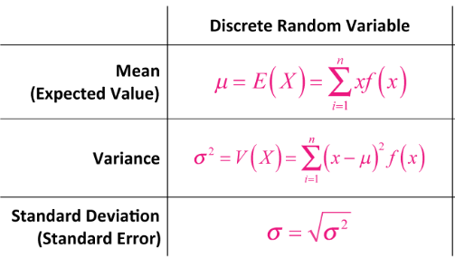
The mean represents the long-run average value if the random process were repeated many times.
- Formula: \( \mu_X = E[X] = \sum x \cdot P(X = x) \).
- Interpretation: Balance point of the probability distribution.
Variance and Standard Deviation
Variance measures how far the values of \( X \) are spread from the mean.
Formula: \( \sigma_X^2 = \sum (x – \mu_X)^2 \cdot P(X = x) \).
Standard deviation is the square root of variance:
Formula: \( \sigma_X = \sqrt{\sigma_X^2} \).
Interpretation: Typical distance of a random variable from its mean.
Example
A random variable \( X \) represents the number of defective bulbs in a box of 3. The probability distribution is:
- \( P(X = 0) = 0.6 \)
- \( P(X = 1) = 0.3 \)
- \( P(X = 2) = 0.1 \)
Find the mean (expected value) of \( X \).
▶️ Answer / Explanation
Step 1: Use formula \( \mu_X = \sum x \cdot P(X = x) \).
Step 2: \( \mu_X = (0)(0.6) + (1)(0.3) + (2)(0.1) \).
Step 3: \( \mu_X = 0 + 0.3 + 0.2 = 0.5 \).
Answer: The mean number of defective bulbs is \( \mu_X = 0.5 \).
Example
Using the same probability distribution:
- \( P(X = 0) = 0.6 \)
- \( P(X = 1) = 0.3 \)
- \( P(X = 2) = 0.1 \)
Find the standard deviation of \( X \).
▶️ Answer / Explanation
Step 1: Recall formula \( \sigma_X^2 = \sum (x – \mu_X)^2 \cdot P(X = x) \).
Step 2: We already found \( \mu_X = 0.5 \).
Step 3: Compute:
- \( (0 – 0.5)^2 (0.6) = 0.25 \times 0.6 = 0.15 \)
- \( (1 – 0.5)^2 (0.3) = 0.25 \times 0.3 = 0.075 \)
- \( (2 – 0.5)^2 (0.1) = 2.25 \times 0.1 = 0.225 \)
Step 4: \( \sigma_X^2 = 0.15 + 0.075 + 0.225 = 0.45 \).
Step 5: \( \sigma_X = \sqrt{0.45} \approx 0.67 \).
Answer: The standard deviation is approximately \( \sigma_X = 0.67 \).
Interpret Parameters of a Discrete Random Variable
Mean ( \( \mu_X \) ):
Represents the expected long-term average of the outcomes. It tells us the “center” of the distribution.
Standard Deviation ( \( \sigma_X \) ):
Measures variability of outcomes. A small standard deviation means outcomes cluster close to the mean; a large one means more spread out.
Individual Probabilities:
Each \( P(X = x) \) shows the likelihood of a specific outcome, helping us interpret what is typical versus unusual.
Unusual Outcomes:
If an outcome lies more than 2 standard deviations away from the mean, it is often considered unusual.
Contextual Meaning: Parameters must be interpreted in the real-world context of the problem (e.g., “On average, 0.5 defective bulbs per box, with a typical variation of 0.67 bulbs”).
Example :
A company produces light bulbs. Let \( X \) be the number of defective bulbs in a randomly selected box of 10 bulbs. The probability distribution of \( X \) has:
- Mean \( \mu_X = 0.5 \)
- Standard deviation \( \sigma_X = 0.67 \)
Interpret the parameters of \( X \) in context.
▶️ Answer / Explanation
- Mean (\( \mu_X = 0.5 \)): On average, there are 0.5 defective bulbs per box of 10. Over many boxes, the long-run average number of defective bulbs will approach 0.5.
- Standard deviation (\( \sigma_X = 0.67 \)): The number of defective bulbs typically varies by about 0.67 from the mean. Most boxes will have between 0 and 1 defective bulbs.
- Unusual outcomes: Values more than 2 standard deviations away (i.e., \( 0.5 \pm 2(0.67) \) → below 0 or above 1.84) are rare. Having 3 or more defective bulbs would be unusual.
Conclusion: The production process is consistent, with few defective bulbs and little variation across boxes.
Example :
Let \( X \) be the number of goals a soccer player scores in a game. The probability distribution of \( X \) is given by:
Goals (\(x\)) | 0 | 1 | 2 | 3 |
---|---|---|---|---|
\( P(X = x) \) | 0.50 | 0.30 | 0.15 | 0.05 |
Using this distribution, \( \mu_X = 0.75 \) and \( \sigma_X \approx 0.90 \).
Interpret the mean and standard deviation in context.
▶️ Answer / Explanation
- Mean (\( \mu_X = 0.75 \)): On average, the player scores about 0.75 goals per game — roughly 3 goals every 4 games.
- Standard deviation (\( \sigma_X = 0.90 \)): The number of goals varies typically by about 0.9 from the average. In most games, the player’s goal count will be between 0 and 2.
- Unusual outcomes: Scores more than 2 SDs above the mean → \( 0.75 + 2(0.90) = 2.55 \). Scoring 3 goals or more is unusual.
Conclusion: The player typically scores between 0–2 goals, with an average close to 1 goal per game. A hat trick (3 goals) is rare and exceptional.