Normal Distributions: Interval Probabilities
In statistics, many real-world variables (like heights, weights, or test scores) follow a normal distribution. We can use the normal model to calculate the probability that a value lies within a given interval.
Key Concepts
Standardization (Z-scores):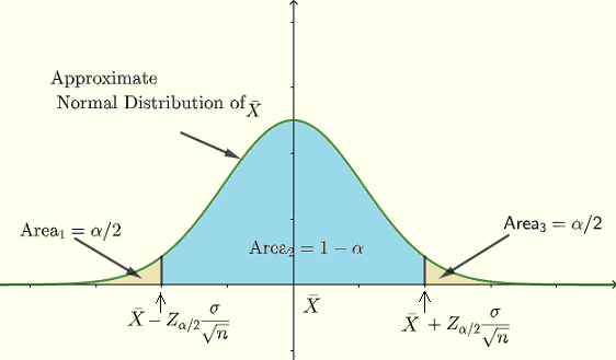
Convert a raw score \( x \) to a standard normal score using \( z = \dfrac{x – \mu}{\sigma} \).
Standard Normal Distribution:
A normal distribution with mean 0 and standard deviation 1.
Probabilities are found using z-tables or technology.
Interval Probabilities:
To find \( P(a \leq X \leq b) \), compute the corresponding z-scores and subtract:
\(P(a \leq X \leq b) = P(Z \leq z_b) – P(Z \leq z_a). \)
Key Takeaways
- Always convert raw values into z-scores before finding probabilities.
- Use technology (normalcdf on calculator, statistical software, or tables) for more accurate results.
- Interval probabilities are found by subtraction: upper probability minus lower probability.
Example
The heights of adult men in a city are normally distributed with mean \( \mu = 70 \) inches and standard deviation \( \sigma = 3 \) inches. What is the probability that a randomly selected man has a height between 68 and 74 inches?
Find \( P(68 \leq X \leq 74) \).
▶️ Answer / Explanation
Step 1: Standardize both values.
- \( z_1 = \dfrac{68 – 70}{3} = \dfrac{-2}{3} \approx -0.67 \)
- \( z_2 = \dfrac{74 – 70}{3} = \dfrac{4}{3} \approx 1.33 \)
Step 2: Find probabilities from the standard normal distribution.
- \( P(Z \leq -0.67) \approx 0.2514 \)
- \( P(Z \leq 1.33) \approx 0.9082 \)
Step 3: Subtract to find the interval probability.
\( P(68 \leq X \leq 74) = 0.9082 – 0.2514 = 0.6568 \).
Answer: The probability is about 65.7% that a randomly selected man has a height between 68 and 74 inches.
Normal Distribution: Intervals from Areas
Intervals in a normal distribution are found by connecting probabilities (areas under the curve) to boundary values of \( x \). These boundaries depend on whether we are interested in the left tail, right tail, middle region, or extreme values.
Left-Tail Interval:
\( P(X < x_a) = \dfrac{p}{100} \)
This means that the lowest \( p\% \) of values lie to the left of \( x_a \).
Example: The 10th percentile is the value below which 10% of observations fall.
Middle Interval:
\( P(x_a < X < x_b) = \dfrac{p}{100} \)
This means that \( p\% \) of values lie between two cutoffs \( x_a \) and \( x_b \).
Example: The middle 80% of values is bounded by the 10th and 90th percentiles.
Right-Tail Interval:
\( P(X > x_b) = \dfrac{p}{100} \)
This means that the highest \( p\% \) of values lie to the right of \( x_b \).
Example: The top 5% cutoff (like elite test scores).
Extreme Tails (Two-Sided):
To capture the most extreme \( p\% \) of values, split into two equal tails:
\( P(X < x_a) = \dfrac{1}{2}\dfrac{p}{100}, \quad P(X > x_b) = \dfrac{1}{2}\dfrac{p}{100} \)
This means half of the \( p\% \) most extreme values lie below \( x_a \), and half lie above \( x_b \).
Example: The most extreme 2% of observations means 1% in each tail.
How to Solve:
- Identify whether the problem is left-tail, right-tail, central, or extreme.
- Translate the probability into the corresponding z-score(s) using tables or technology.
- Convert back to raw scores with: \( x = \mu + z \cdot \sigma \).
Example
The scores on a standardized test are normally distributed with mean \( \mu = 500 \) and standard deviation \( \sigma = 100 \). Find the test score that marks the 90th percentile.
What value of \( x \) corresponds to the top 10% cutoff?
▶️ Answer / Explanation
Step 1: The 90th percentile means \( P(X \leq x) = 0.90 \).
Step 2: From z-tables or technology, \( z_{0.90} \approx 1.28 \).
Step 3: Convert back to raw score: \( x = \mu + z \cdot \sigma = 500 + (1.28)(100) = 628 \).
Answer: The 90th percentile score is approximately 628.
Example
The weights of bags of chips are normally distributed with mean \( \mu = 14 \) oz and standard deviation \( \sigma = 0.3 \) oz. Find the interval that contains the middle 95% of all bag weights.
What interval \( (a, b) \) contains the middle 95% of weights?
▶️ Answer / Explanation
Step 1: Middle 95% leaves 2.5% in each tail.
Step 2: Critical z-scores: \( z = \pm 1.96 \).
Step 3: Convert back to raw values:
- Lower bound: \( a = 14 + (-1.96)(0.3) = 14 – 0.588 \approx 13.41 \)
- Upper bound: \( b = 14 + (1.96)(0.3) = 14 + 0.588 \approx 14.59 \)
Answer: The middle 95% of bag weights lie between 13.41 oz and 14.59 oz.