AP Statistics 5.3 The Central Limit Theorem Study Notes

Sampling Distributions and the Central Limit Theorem

 Sampling Distribution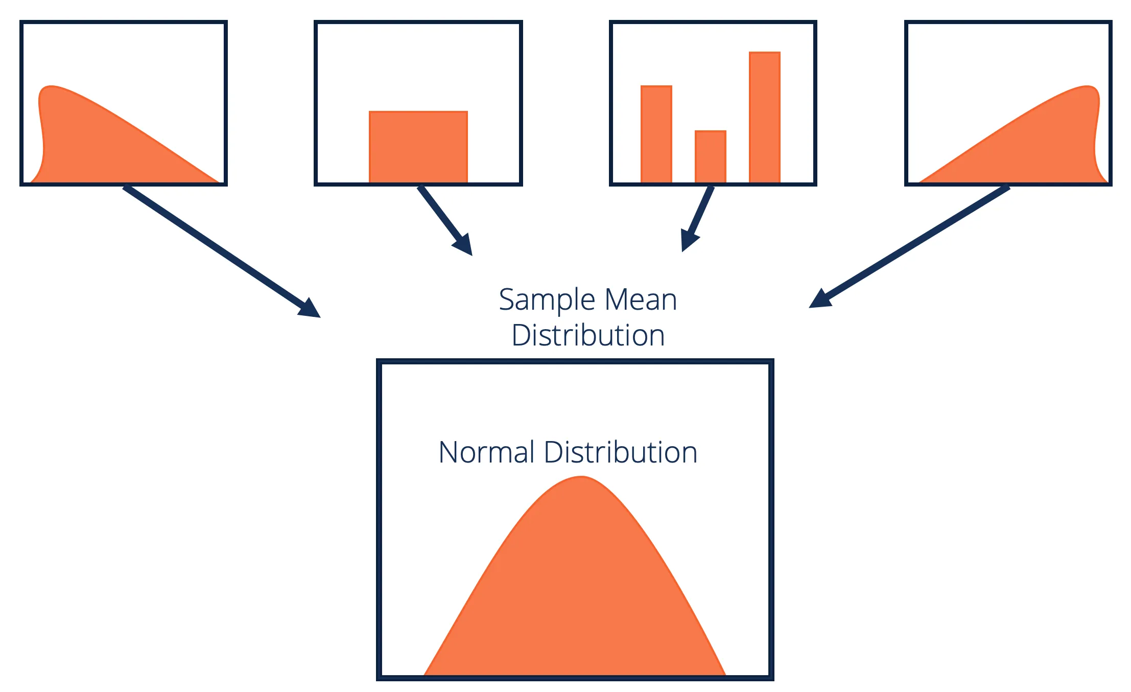

A sampling distribution is the probability distribution of a statistic (such as the sample mean, sample proportion, or sample variance) based on all possible random samples of a fixed size taken from the same population.

• It shows how the statistic would vary if we repeatedly took samples of the same size.
• The variability of a sampling distribution decreases as sample size increases because larger samples reduce sampling error.

Example: If we take many samples of size \( n = 50 \) from a population with mean \( \mu = 100 \), the average values from each sample will not be identical, but their distribution forms the sampling distribution of the sample mean.

Central Limit Theorem (CLT)

The CLT states that if the sample size is sufficiently large, the sampling distribution of the sample mean \( \bar{X} \) will be approximately normal, regardless of the population’s distribution.

Parameters of the Sampling Distribution of the Mean:

• • Mean: \( \mu_{\bar{X}} = \mu \) (the mean of the sample means equals the population mean).
  • Standard Deviation (Standard Error): \( \sigma_{\bar{X}} = \dfrac{\sigma}{\sqrt{n}} \), where \( \sigma \) is the population standard deviation and \( n \) is the sample size.
• As \( n \) increases, the sampling distribution becomes more tightly clustered around the population mean.

Example: Even if exam scores in a class are skewed, the distribution of average scores from many random samples of 40 students will look approximately normal.

Conditions for the CLT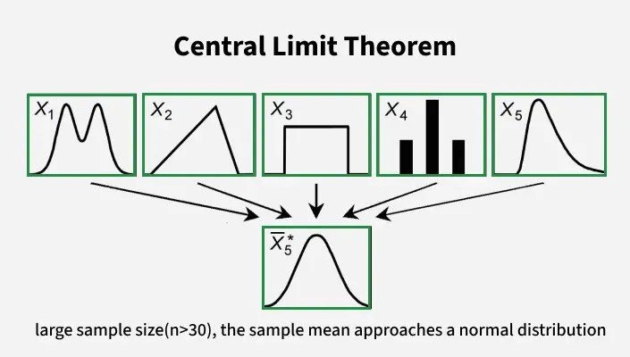

• Independence: The sampled values must be independent. This is usually satisfied if sampling is random and the population is large relative to the sample size (rule of thumb: population at least 10 times the sample size).
• Sample Size: The sample size must be sufficiently large.
  • If the population distribution is normal, any sample size works.
  • If the population is not normal, \( n \geq 30 \) is usually considered large enough.

 Randomization Distribution

A randomization distribution is created by simulating the process of random assignment under the assumption that the null hypothesis is true.

• For experiments, this involves repeatedly and randomly reallocating the observed responses to treatment groups to see what kinds of differences could occur just by chance.
• This forms the basis for significance testing: if the observed statistic is very unlikely compared to this randomization distribution, we conclude that the treatment had an effect.

Example: In a drug experiment, we could shuffle “improvement” responses among treatment and placebo groups thousands of times to build a randomization distribution of differences in means.

 Simulating a Sampling Distribution

When it is impractical to calculate a theoretical sampling distribution, we can use computer simulation to approximate it.

• The process:
  1. Take a random sample from the population.
  2. Compute the statistic of interest (e.g., mean, proportion).
  3. Repeat steps 1 and 2 many times (hundreds or thousands).
  4. Plot the distribution of these statistics. This approximates the sampling distribution.

Example: If we simulate rolling a fair die 50 times and calculate the average, then repeat this 1,000 times, the distribution of those averages will be approximately normal (by the CLT).