Explain why an estimator is or is not unbiased
Unbiased Estimator: An estimator is unbiased if the expected value of the statistic equals the true population parameter. That is, \( E(\hat{\theta}) = \theta \). This means that, on average over many samples, the estimator correctly targets the population parameter.
Biased Estimator: An estimator is biased if the expected value does not equal the population parameter. That is, \( E(\hat{\theta}) \neq \theta \). This means the estimator systematically overestimates or underestimates the true parameter.
Common Examples: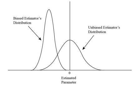
- Sample mean \( \bar{x} \) is an unbiased estimator of the population mean \( \mu \).
- Sample proportion \( \hat{p} \) is an unbiased estimator of the population proportion \( p \).
- Sample variance using denominator \( n-1 \) is an unbiased estimator of population variance \( \sigma^2 \). Using denominator \( n \) instead is biased (tends to underestimate).
Visual Analogy:
Think of aiming at a target:
- Unbiased: The arrows cluster around the bullseye (correct on average, even with some spread).
- Biased: The arrows cluster away from the bullseye (systematic error).
Example
Suppose a population has mean \( \mu = 50 \). You take many random samples of size \( n = 30 \) and compute the sample mean \( \bar{x} \) for each. Question: Is \( \bar{x} \) an unbiased estimator of \( \mu \)?
▶️ Answer / Explanation
The expected value of \( \bar{x} \) is equal to \( \mu \), i.e. \( E(\bar{x}) = \mu = 50 \). Over many repeated samples, the average of the sample means will equal the true population mean.
Conclusion: \( \bar{x} \) is an unbiased estimator of \( \mu \).
Example
A researcher estimates population variance \( \sigma^2 \) using the formula: \[ s_n^2 = \dfrac{1}{n} \sum (x_i – \bar{x})^2 \] instead of dividing by \( n-1 \). Question: Is this estimator unbiased?
▶️ Answer / Explanation
For finite samples, using denominator \( n \) underestimates \( \sigma^2 \) because it does not fully account for the variability lost by using \( \bar{x} \) as an estimate of \( \mu \). Thus, \( E(s_n^2) < \sigma^2 \).
Conclusion: \( s_n^2 \) is a biased estimator of \( \sigma^2 \).
Example
A poll asks 500 people if they like a new product. Let \( \hat{p} \) be the proportion who say “yes.” Question: Is \( \hat{p} \) an unbiased estimator of the true population proportion \( p \)?
▶️ Answer / Explanation
The expected value of \( \hat{p} \) is equal to the population proportion: \( E(\hat{p}) = p \). Across many samples, the average sample proportion equals the true population proportion.
Conclusion: \( \hat{p} \) is an unbiased estimator of \( p \).
Calculate Estimates for a Population Parameter
Point Estimate: A single value used to approximate a population parameter.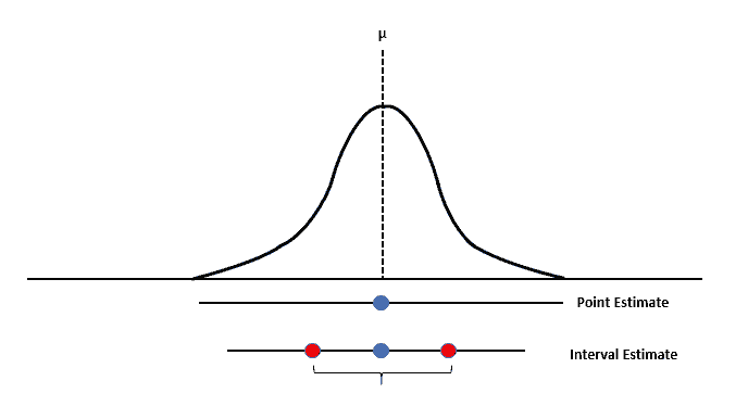
Examples:
- \( \bar{x} \) estimates population mean \( \mu \).
- \( \hat{p} \) estimates population proportion \( p \).
Interval Estimate: An interval of values (confidence interval) that is likely to contain the population parameter. Example: A 95% confidence interval for the mean test score.
Key Ideas:
- The goal is to use sample statistics to estimate unknown population parameters.
- Point estimates are useful but can vary from sample to sample (sampling variability).
- Interval estimates provide a range with a certain level of confidence.
- Larger samples tend to give more precise (less variable) estimates.
Comparison Table
| Population Parameter | Sample Statistic (Estimator) | Type of Estimate |
|---|---|---|
| Population Mean \( \mu \) | Sample Mean \( \bar{x} \) | Point Estimate |
| Population Proportion \( p \) | Sample Proportion \( \hat{p} \) | Point Estimate |
| Population Mean \( \mu \) | Confidence Interval for \( \mu \) | Interval Estimate |
| Population Proportion \( p \) | Confidence Interval for \( p \) | Interval Estimate |
Example
A random sample of 40 students has an average study time of \( \bar{x} = 3.2 \) hours per day. What is the point estimate of the population mean study time \( \mu \)?
▶️ Answer / Explanation
Step 1: The population parameter of interest is the mean \( \mu \).
Step 2: The sample mean \( \bar{x} = 3.2 \) is the point estimate.
Answer: The point estimate of \( \mu \) is \( \bar{x} = 3.2 \) hours.
Example
Out of 200 voters surveyed, 124 say they will support a particular candidate. What is the point estimate of the population proportion \( p \) of voters who support the candidate?
▶️ Answer / Explanation
Step 1: The population parameter of interest is the proportion \( p \).
Step 2: The sample proportion is:
\( \hat{p} = \dfrac{124}{200} = 0.62 \).
Answer: The point estimate of \( p \) is \( \hat{p} = 0.62 \).
Example
A random sample of 50 light bulbs has a mean lifetime of 820 hours and standard deviation of 60 hours. Construct a 95% confidence interval for the population mean lifetime \( \mu \).
▶️ Answer / Explanation
Step 1: The parameter of interest is \( \mu \).
Step 2: Standard error: \( SE = \dfrac{s}{\sqrt{n}} = \dfrac{60}{\sqrt{50}} \approx 8.49 \).
Step 3: For 95% CI, use critical value \( z^* \approx 1.96 \).
Step 4: Margin of error: \( ME = 1.96 \times 8.49 \approx 16.64 \).
Step 5: Interval: \( 820 \pm 16.64 \), or \( (803.36, 836.64) \).
Answer: The 95% confidence interval is approximately \( (803, 837) \) hours.