
5.4.A.1 Residuals
After using a linear regression model to predict a response value, statisticians often compare the observed response value with the predicted response value.
The difference between these two values is called the residual.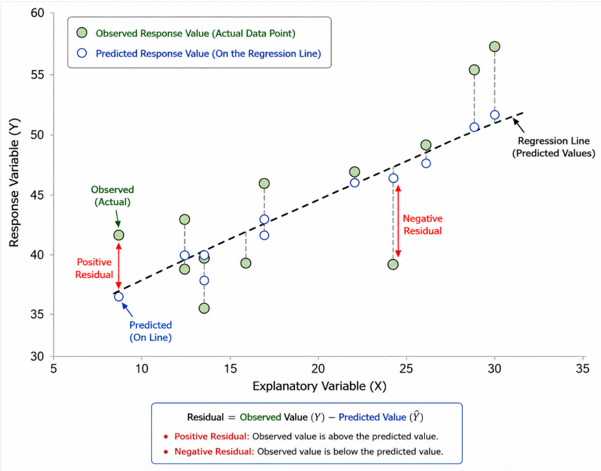
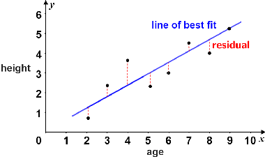
A residual measures how far an observed data point is from the value predicted by the least-squares regression line.
Residual Formula
\( \mathrm{Residual}=y-\hat{y} \)
or
\( \mathrm{Residual}=\mathrm{Observed\ Value}-\mathrm{Predicted\ Value} \)
Where:
- \( y \) = Observed (actual) response value
- \( \hat{y} \) = Predicted response value obtained from the regression equation
- Residual = Difference between the observed and predicted values
Interpreting Residuals
| Residual | Interpretation |
|---|---|
| Positive (\( >0 \)) | The observed value is greater than the predicted value. The regression line underestimates the response. |
| Negative (\( <0 \)) | The observed value is less than the predicted value. The regression line overestimates the response. |
| Zero (\( =0 \)) | The observed value equals the predicted value. The point lies exactly on the regression line. |
Steps for Calculating a Residual
- Use the regression equation to calculate the predicted value \( \hat{y} \).
- Find the observed value \( y \).
- Subtract the predicted value from the observed value.
- Interpret the sign of the residual.
Important AP Exam Notes
- A residual measures the prediction error for a single observation.
- A positive residual indicates that the regression model underestimated the response value.
- A negative residual indicates that the regression model overestimated the response value.
- Residuals are always calculated as Observed − Predicted, never Predicted − Observed.
Example
The least-squares regression equation relating hours studied to mathematics test score is
\( \hat{y}=48+4x \)
A student studied 7 hours and earned an actual score of 79.
Calculate the residual and interpret its meaning.
▶️ Answer / Explanation
Step 1: Calculate the predicted score.
\( \hat{y}=48+4(7)=76 \)
Step 2: Calculate the residual.
\( \mathrm{Residual}=79-76=3 \)
The residual is \( 3 \).
Because the residual is positive, the student’s actual mathematics test score was 3 points higher than the value predicted by the regression model. Therefore, the regression line underestimated the student’s score.
5.4.B.1 Interpreting Residuals
After calculating a residual, statisticians interpret its value to determine whether the linear regression model underpredicted or overpredicted the response variable.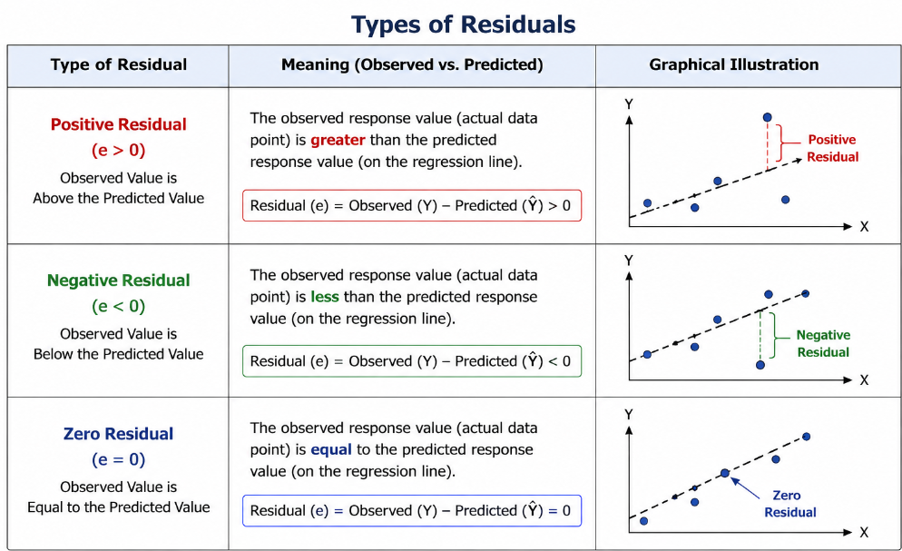
Recall that a residual is calculated as the difference between the observed response value and the predicted response value.
Residual Formula
\( \mathrm{Residual}=y-\hat{y} \)
or
\( \mathrm{Residual}=\mathrm{Observed\ Value}-\mathrm{Predicted\ Value} \)
Interpreting the Sign of a Residual
| Residual | Model Interpretation | Reason |
|---|---|---|
| Positive (\( >0 \)) | The model underpredicts (underestimates) the response variable. | The observed value is greater than the predicted value. |
| Negative (\( <0 \)) | The model overpredicts (overestimates) the response variable. | The predicted value is greater than the observed value. |
| Zero (\( =0 \)) | The model predicts the response exactly. | The observed value equals the predicted value. |
Important AP Exam Notes
- A positive residual means the actual (observed) response is greater than the predicted response.
- A negative residual means the actual (observed) response is less than the predicted response.
- A residual of 0 means the observed value lies exactly on the least-squares regression line.
- Always interpret the residual in the context of the problem.
- Remember that residuals are calculated as Observed − Predicted.
Example
A least-squares regression model predicts that a student who studies 6 hours should earn a mathematics test score of 82.
The student’s actual test score is 78.
Calculate the residual and interpret its meaning.
▶️ Answer / Explanation
Step 1: Calculate the residual.
\( \mathrm{Residual}=78-82=-4 \)
Step 2: Interpret the residual.
The residual is \( -4 \), which is negative.
This means the regression model overpredicted (overestimated) the student’s mathematics test score by 4 points. The actual score was 4 points lower than the predicted score.
5.4.C.1 Residual Plots
After fitting a linear regression model, statisticians use a residual plot to evaluate how well the regression line fits the observed data.
A residual plot is a scatterplot that displays the residuals for each observation against either:
- The predicted response values (\( \hat{y} \)), or
- The explanatory variable values (\( x \)).
Each point on a residual plot represents one observation from the original data set.
The vertical coordinate is the residual, which is calculated as
\( \mathrm{Residual}=y-\hat{y} \)
The horizontal coordinate is either the predicted response value \( \hat{y} \) or the explanatory variable value \( x \).
Unlike the original scatterplot, a residual plot focuses on the prediction errors made by the regression model rather than the original data values.
| Original Scatterplot | Residual Plot |
|---|---|
| Displays the relationship between the explanatory and response variables. | Displays the residuals versus the predicted response values or explanatory variable values. |
| Shows the overall trend of the data. | Shows how far each observed value is from the regression line. |
| Used to identify the form of the relationship. | Used to evaluate how well the regression model fits the data. |
5.4.C.2 Using Residual Plots to Evaluate a Linear Regression Model
Residual plots help statisticians determine whether a linear regression model is appropriate for the observed data.
Because residuals measure the prediction errors of the regression model, the pattern of points in a residual plot reveals whether the linear model adequately describes the relationship.
A residual plot should always be examined after fitting a regression line because the value of the correlation coefficient alone cannot determine whether a linear model is appropriate.
Residual plots are useful for:
- Evaluating the appropriateness of a linear regression model.
- Detecting non-linear relationships.
- Identifying unusual observations or outliers.
- Checking whether the residuals display any systematic pattern.
Important AP Exam Notes
- A residual plot evaluates the fit of a regression model, not the strength of the association.
- The points in a residual plot should be examined for patterns.
- A clear pattern in the residuals often suggests that the linear model does not adequately describe the data.
- Residual plots provide evidence about whether a linear regression model is appropriate.
Example
A statistician fits a least-squares regression line to data relating weekly study time and mathematics test scores.
To determine whether the linear regression model is appropriate, the statistician constructs a residual plot.
Explain why a residual plot is useful after fitting a regression model.
▶️ Answer / Explanation
A residual plot displays the prediction errors made by the regression model.
By examining the pattern of the residuals, a statistician can determine whether the linear regression model adequately represents the data or whether another model may be more appropriate.
If the residual plot shows a systematic pattern, the linear model may not be suitable for the data.
5.4.C.3 Interpreting Residual Plots for a Linear Regression Model
A residual plot helps determine whether a linear regression model is appropriate for a set of bivariate quantitative data.
The linear regression model should be used only if the relationship between the explanatory and response variables is approximately linear.
If the residual plot shows an apparently random scatter of points around the horizontal line at \( \mathrm{Residual}=0 \), then the linear model is appropriate.
A random pattern indicates that the regression model has accounted for the linear trend in the data and that no systematic pattern remains in the residuals.
Random Residual Plot
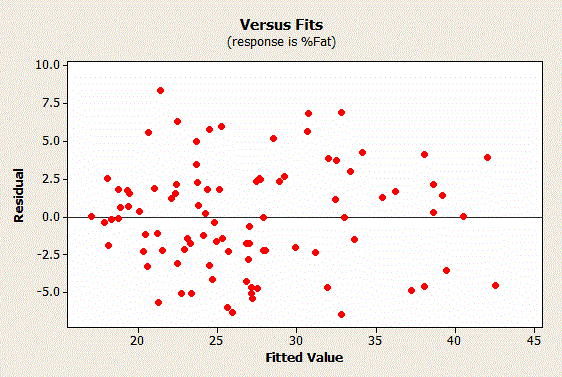
- The residuals are randomly scattered above and below \( \mathrm{Residual}=0 \).
- No obvious pattern or trend is present.
- The spread of the residuals is approximately constant.
- This provides evidence that a simple linear regression model is appropriate.
| Residual Plot Pattern | Interpretation |
|---|---|
| Random scatter about \( \mathrm{Residual}=0 \) | The linear regression model is appropriate. |
| No systematic pattern | The residuals support a linear form for the association. |
5.4.C.4 Curvature in a Residual Plot
If the residual plot displays a noticeable curved pattern, the residuals are not randomly distributed.
This indicates that the linear regression model has failed to capture an important feature of the relationship between the variables.
A curved residual plot suggests that the relationship between the variables is non-linear, and a different model may better describe the data.
Curved Residual Plot
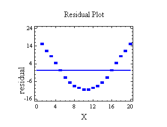
- The residuals form a curved or systematic pattern.
- The points are not randomly scattered around zero.
- The relationship between the variables is likely non-linear.
- A simple linear regression model is not the most appropriate model.
| Residual Plot | Conclusion |
|---|---|
| Random scatter around zero | A linear regression model is appropriate. |
| Curved or systematic pattern | A linear regression model is not appropriate. |
| Distinct pattern remaining in the residuals | Another regression model should be considered. |
Important AP Exam Notes
- A random residual plot confirms that a linear model is appropriate.
- A curved residual plot suggests that the relationship is non-linear.
- Residual plots should always be interpreted together with the original scatterplot.
- When describing a residual plot, focus on whether the residuals are random or show a systematic pattern.
Example
A residual plot for a least-squares regression model shows the residuals randomly scattered above and below the horizontal line at \( \mathrm{Residual}=0 \), with no noticeable pattern.
Determine whether a linear regression model is appropriate and justify your answer.
▶️ Answer / Explanation
The residual plot displays a random scatter of points around the horizontal line at \( \mathrm{Residual}=0 \).
Because there is no systematic pattern or curvature in the residuals, the plot provides evidence that the relationship between the variables is approximately linear.
Therefore, a simple linear regression model is appropriate for describing the data.