
5.5.A.1 Least-Squares Regression Line (LSRL)
When the relationship between two quantitative variables appears to be approximately linear, statisticians use a simple linear regression model to describe the relationship and predict values of the response variable.
The regression line is chosen so that it provides the best possible linear fit to the observed data.
This line is called the Least-Squares Regression Line (LSRL) because it is determined by minimizing the sum of the squared residuals.
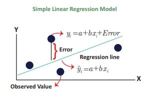
A residual is the difference between the observed response value and the predicted response value.
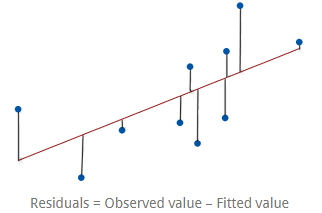
\( \mathrm{Residual}=y-\hat{y} \)
Since some residuals are positive and others are negative, simply adding them together could produce a value close to zero. To prevent positive and negative residuals from canceling each other out, each residual is squared before being added.
The Least-Squares Regression Line is the line for which the sum of the squared residuals is as small as possible.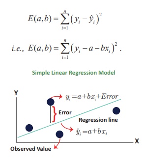
Least-Squares Criterion
\( \mathrm{Minimize}\ \sum (y-\hat{y})^{2} \)
where
- \( y \) = Observed response value
- \( \hat{y} \) = Predicted response value
- \( y-\hat{y} \) = Residual
- \( \sum (y-\hat{y})^{2} \) = Sum of the squared residuals
Because finding the least-squares regression line requires many calculations, the equation is almost always determined using technology, such as a graphing calculator or statistical software.
The equation of the Least-Squares Regression Line is
\( \hat{y}=a+bx \)
where
- \( \hat{y} \) = Predicted response value
- \( a \) = y-intercept of the regression line
- \( b \) = Slope of the regression line
- \( x \) = Explanatory variable
An Important Property of the LSRL
The Least-Squares Regression Line always passes through the point
\( (\bar{x},\bar{y}) \)
where
- \( \bar{x} \) = Mean of the explanatory variable
- \( \bar{y} \) = Mean of the response variable
This means that the average values of the explanatory and response variables always lie on the regression line.
| Concept | Description |
|---|---|
| Least-Squares Regression Line (LSRL) | The line that minimizes the sum of the squared residuals. |
| Residual | Difference between the observed and predicted response values. |
| Least-Squares Criterion | Chooses the regression line with the smallest value of \( \sum (y-\hat{y})^{2} \). |
| Special Property | The regression line always passes through \( (\bar{x},\bar{y}) \). |
| Calculation | The LSRL is calculated using technology. |
Important AP Exam Notes
- The Least-Squares Regression Line is the best-fitting linear model because it minimizes the sum of the squared residuals.
- The equation of the LSRL is determined using technology; students are not expected to calculate it by hand.
- The regression line always passes through the point \( (\bar{x},\bar{y}) \).
- Minimizing the sum of the squared residuals produces the line with the smallest overall prediction error.
Example
A researcher collects data relating the number of hours students study each week to their mathematics test scores. A graphing calculator is used to determine the Least-Squares Regression Line.
Why is the regression line called the Least-Squares Regression Line (LSRL)?
▶️ Answer / Explanation
The regression line is called the Least-Squares Regression Line because it is the line that minimizes the sum of the squared residuals.
Each residual is the difference between an observed response value and its predicted response value. Squaring the residuals prevents positive and negative residuals from canceling each other out.
The resulting line provides the best-fitting linear model for the observed data and always passes through the point \( (\bar{x},\bar{y}) \).
Example
A statistician collected data on the number of hours students studied and their mathematics test scores. A graphing calculator produced the following least-squares regression line:
\( \hat{y}=42+5x \)
The mean number of hours studied is
\( \bar{x}=6 \)
Verify that the Least-Squares Regression Line passes through the point \( (\bar{x},\bar{y}) \) by finding \( \bar{y} \).
▶️ Answer / Explanation
Since the Least-Squares Regression Line always passes through \( (\bar{x},\bar{y}) \), substitute \( \bar{x}=6 \) into the regression equation.
\( \hat{y}=42+5(6) \)
\( \hat{y}=42+30 \)
\( \hat{y}=72 \)
Therefore,
\( \bar{y}=72 \)
Hence, the Least-Squares Regression Line passes through the point
\( (\bar{x},\bar{y})=(6,\;72) \)
This confirms the important property that every Least-Squares Regression Line passes through the point formed by the mean of the explanatory variable and the mean of the response variable.
5.5.A.2 Slope of the Least-Squares Regression Line
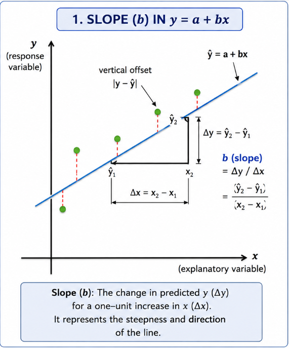
The slope of the least-squares regression line describes how the predicted response variable changes for each one-unit increase in the explanatory variable.
In the regression equation
\( \hat{y}=a+bx \)
the coefficient \( b \) represents the slope of the regression line.
The slope is calculated using technology, such as a graphing calculator or statistical software.
Interpreting the Slope
The slope represents the predicted change in the response variable for every one-unit increase in the explanatory variable.
| Slope (\( b \)) | Interpretation |
|---|---|
| \( b>0 \) | As the explanatory variable increases, the predicted response variable increases. |
| \( b<0 \) | As the explanatory variable increases, the predicted response variable decreases. |
| \( b=0 \) | The regression line is horizontal, indicating no linear trend. |
Important AP Exam Notes
- The slope is interpreted in the context of the variables.
- The slope describes the change in the predicted response variable, not necessarily the observed value.
- The value of the slope is calculated using technology.
Example
The least-squares regression equation relating hours studied (\( x \)) to mathematics test score (\( y \)) is
\( \hat{y}=48+4x \)
Interpret the slope of the regression line.
▶️ Answer / Explanation
The slope is 4.
For every additional hour a student studies, the predicted mathematics test score increases by approximately 4 points, on average.
5.5.A.3 y-Intercept of the Least-Squares Regression Line
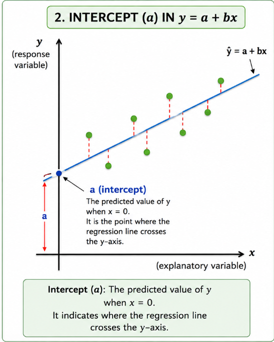
The y-intercept of the least-squares regression line is the predicted value of the response variable when the explanatory variable is equal to \( 0 \).
In the regression equation
\( \hat{y}=a+bx \)
the coefficient \( a \) represents the y-intercept.
The y-intercept is calculated using technology.
Interpreting the y-Intercept
The y-intercept represents the predicted response value when
\( x=0 \)
However, the y-intercept should only be interpreted if \( x=0 \) is meaningful in the context of the data.
| Coefficient | Meaning |
|---|---|
| \( a \) | Predicted value of the response variable when \( x=0 \). |
Important AP Exam Notes
- The y-intercept is not always meaningful.
- If \( x=0 \) is outside the range of the observed data, the y-intercept may have little practical interpretation.
- The y-intercept is calculated using technology.
Example
The least-squares regression equation relating hours studied to mathematics test score is
\( \hat{y}=48+4x \)
Interpret the y-intercept.
▶️ Answer / Explanation
The y-intercept is 48.
According to the regression model, a student who studies 0 hours is predicted to score 48 points on the mathematics test.
This interpretation is meaningful only if studying 0 hours is a reasonable value within the context of the data.
5.5.A.4 Correlation Coefficient (\( r \))
In simple linear regression, the correlation coefficient, denoted by \( r \), measures the strength and direction of the linear relationship between two quantitative variables.
The correlation coefficient is calculated using technology.
The value of \( r \) always satisfies
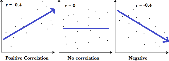
\( -1\le r\le1 \)
| Value of \( r \) | Interpretation |
|---|---|
| Positive | Positive linear association. |
| Negative | Negative linear association. |
| Close to ±1 | Strong linear association. |
| Close to 0 | Weak or no linear association. |
Important AP Exam Notes
- The value of \( r \) is always calculated using technology.
- The sign of \( r \) indicates the direction of the association.
- The magnitude of \( r \) indicates the strength of the linear association.
- The correlation coefficient has no units.
Example
A graphing calculator reports the following value for a linear regression analysis:
\( r=-0.91 \)
Interpret the correlation coefficient.
▶️ Answer / Explanation
Because \( r=-0.91 \) is negative, the variables have a negative linear association.
Since the value is close to \( -1 \), the association is strong.
Therefore, there is a strong negative linear relationship between the two quantitative variables.
Example
The table below shows the number of hours students studied for an exam and their corresponding mathematics test scores.
| Hours Studied (\(x\)) | Test Score (\(y\)) |
|---|---|
| 2 | 58 |
| 4 | 65 |
| 5 | 70 |
| 7 | 78 |
| 9 | 86 |
Using technology, calculate the following:
- The Least-Squares Regression Line (LSRL).
- The slope (\(b\)).
- The y-intercept (\(a\)).
- The correlation coefficient (\(r\)).
▶️ Answer / Explanation
Step 1: Enter the data into the calculator.
- Enter the \(x\)-values into L1.
- Enter the \(y\)-values into L2.
Step 2: Perform Linear Regression.
On a TI-84 calculator:
STAT → CALC → LinReg(ax+b) (or LinReg(a+bx)) → L1, L2 → Calculate
Step 3: Read the calculator output.
The calculator reports approximately:
Slope ((b)) = (4.06)
y-intercept ((a)) = (49.83)
Correlation coefficient ((r)) = (0.997)
Step 4: Write the regression equation.
( \hat{y}=49.83+4.06x )
Interpretation
- The slope indicates that for every additional hour studied, the predicted mathematics test score increases by approximately 4.06 points.
- The y-intercept indicates that a student who studies 0 hours is predicted to score about 49.83 points (if meaningful in context).
- The correlation coefficient \(r=0.997\) indicates a very strong positive linear association between hours studied and mathematics test score.
5.5.A.5 Coefficient of Determination (\( r^2 \))
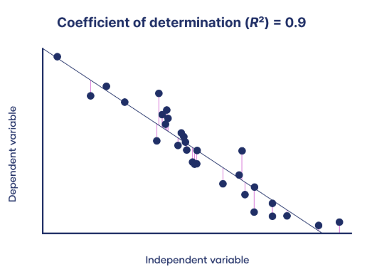
In simple linear regression, the square of the correlation coefficient, denoted by \( r^2 \), is called the coefficient of determination.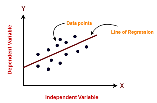
The coefficient of determination measures how well the least-squares regression line explains the variation in the response variable.
Formula
\( r^2=(r)^2 \)
where
- \( r \) = Correlation coefficient
- \( r^2 \) = Coefficient of determination
The value of \( r^2 \) represents the proportion (or percentage) of the variation in the response variable that is explained by the linear relationship with the explanatory variable.
The remaining variation is due to other factors or random variability that is not explained by the regression model.
| Value of \(r^2\) | Interpretation |
|---|---|
| \(0\) | The linear model explains none of the variation in the response variable. |
| Between \(0\) and \(1\) | The linear model explains a proportion of the variation in the response variable. |
| \(1\) | The linear model explains all of the variation in the response variable. |
Important AP Exam Notes
- \( r^2 \) is called the coefficient of determination.
- \( r^2 \) is always between 0 and 1.
- Multiply \( r^2 \) by 100% to express the explained variation as a percentage.
- The remaining variation, \(1-r^2\), represents the proportion of variation not explained by the linear regression model.
- Always interpret \( r^2 \) in the context of the response variable.
Example
A linear regression analysis relating hours studied (\(x\)) to mathematics test scores (\(y\)) produced a correlation coefficient of
\( r=0.90 \)
Calculate the coefficient of determination and interpret its meaning.
▶️ Answer / Explanation
Step 1: Calculate \(r^2\).
\( r^2=(0.90)^2=0.81 \)
Step 2: Convert to a percentage.
\( 0.81\times100\%=81\% \)
Interpretation:
Approximately 81% of the variation in mathematics test scores is explained by the linear relationship with hours studied.
The remaining 19% of the variation is due to other factors or random variation that are not explained by the linear regression model.
5.5.B.1 Coefficients of the Least-Squares Regression Line
The Least-Squares Regression Line (LSRL), also called the line of best fit, is used to model the linear relationship between an explanatory variable and a response variable.
The equation of the Least-Squares Regression Line is
\( \hat{y}=a+bx \)
The two numerical values in the regression equation are called the coefficients of the least-squares regression line.
The coefficients are:
- \(a\) = y-intercept
- \(b\) = slope
Because the regression line is constructed using sample data, the values of \(a\) and \(b\) are statistics, not parameters.
These coefficients summarize the linear relationship between the explanatory and response variables and are calculated using technology.
| Coefficient | Symbol | Meaning |
|---|---|---|
| Slope | \(b\) | Represents the predicted change in the response variable for each one-unit increase in the explanatory variable. |
| y-intercept | \(a\) | Represents the predicted value of the response variable when the explanatory variable is equal to \(0\). |
Important AP Exam Notes
- The coefficients of the LSRL are the slope (\(b\)) and the y-intercept (\(a\)).
- Since the regression line is based on a sample, the coefficients are statistics.
- The coefficients are calculated using technology, such as a graphing calculator or statistical software.
- The coefficients describe the linear relationship between the explanatory and response variables.
Example
A graphing calculator produces the following least-squares regression equation relating hours studied (\(x\)) to mathematics test score (\(y\)):
\( \hat{y}=52.6+3.8x \)
Identify the coefficients of the least-squares regression line.
▶️ Answer / Explanation
The regression equation is
\( \hat{y}=52.6+3.8x \)
Therefore, the coefficients are:
- y-intercept: \(a=52.6\)
- Slope: \(b=3.8\)
These coefficients were calculated from the sample data using technology and define the least-squares regression line.
5.5.B.2 Interpreting the Slope of the Least-Squares Regression Line
The slope of the least-squares regression line describes how the predicted response variable changes for each one-unit increase in the explanatory variable.
In the regression equation
\( \hat{y}=a+bx \)
the coefficient \(b\) represents the slope of the regression line.
The slope indicates the predicted increase or decrease in the response variable for every one-unit increase in the explanatory variable.
The interpretation of the slope should always be written in the context of the variables being studied.
| Value of the Slope | Interpretation |
|---|---|
| \(b>0\) | For each one-unit increase in the explanatory variable, the predicted response variable increases by \(b\) units. |
| \(b<0\) | For each one-unit increase in the explanatory variable, the predicted response variable decreases by \(|b|\) units. |
| \(b=0\) | There is no predicted linear change in the response variable. |
General Interpretation Template
For every one-unit increase in the explanatory variable, the predicted value of the response variable increases (or decreases) by \(b\) units, on average.
Important AP Exam Notes
- Always interpret the slope using the word predicted.
- The slope describes the change in the response variable, not the explanatory variable.
- Interpret the slope in context using the names and units of the variables.
- A positive slope indicates an increasing linear relationship, while a negative slope indicates a decreasing linear relationship.
Example
A least-squares regression equation relating weekly study time (\(x\)) to mathematics test score (\(y\)) is
\( \hat{y}=46.5+5.2x \)
Interpret the slope of the regression line.
▶️ Answer / Explanation
The slope of the regression line is
\( b=5.2 \)
For every additional 1 hour a student studies each week, the predicted mathematics test score increases by approximately 5.2 points, on average.
Because the slope is positive, the regression model predicts that students who study more tend to earn higher mathematics test scores.
5.5.B.3 Interpreting the y-Intercept of the Least-Squares Regression Line
The y-intercept of the least-squares regression line is the predicted value of the response variable when the explanatory variable is equal to \(0\).
In the regression equation
\( \hat{y}=a+bx \)
the coefficient \(a\) represents the y-intercept.
The interpretation of the y-intercept should always be written in the context of the variables being studied.
However, the y-intercept is not always meaningful. Before interpreting it, determine whether the value \(x=0\) is reasonable in the context of the data.
| Situation | Can the y-Intercept Be Interpreted? |
|---|---|
| \(x=0\) is within the observed range of the data and makes sense in context. | Yes. Interpret the y-intercept as the predicted value of the response variable when \(x=0\). |
| \(x=0\) is outside the observed range of the data. | No. Interpreting the y-intercept would require extrapolation. |
| The predicted value at \(x=0\) is not logical in context (for example, a negative height). | No. The y-intercept has no practical interpretation. |
General Interpretation Template
When the explanatory variable is equal to \(0\), the model predicts that the response variable will be approximately \(a\) units.
Important AP Exam Notes
- Always interpret the y-intercept as a predicted value.
- Before interpreting the y-intercept, determine whether \(x=0\) is meaningful in the context of the problem.
- If \(x=0\) is outside the observed range of the data, interpreting the y-intercept involves extrapolation and is generally not appropriate.
- If the predicted value is not realistic (such as a negative height or negative age), the y-intercept should not be interpreted.
Example
A least-squares regression equation relating weekly study time (\(x\)) to mathematics test score (\(y\)) is
\( \hat{y}=48+4x \)
Interpret the y-intercept of the regression line.
▶️ Answer / Explanation
The y-intercept is
\( a=48 \)
This means that a student who studies 0 hours per week is predicted to earn a mathematics test score of approximately 48 points.
This interpretation is appropriate only if studying 0 hours is a reasonable value within the context of the data.