Home / AP Statistics 5.5 Sampling Distributions for Sample Proportions Study Notes

AP Statistics 5.5 Sampling Distributions for Sample Proportions Study Notes

AP Statistics 5.5 Sampling Distributions for Sample Proportions Study Notes- New syllabus

AP Statistics 5.5 Sampling Distributions for Sample Proportions Study Notes -As per latest AP Statistics Syllabus.

LEARNING OBJECTIVE

  • Probabilistic reasoning allows us to anticipate patterns in data.

Key Concepts:

  • Sampling Distributions for Sample Proportions
  • Normal Approximation for a Sample Proportion
  • Interpreting a Sampling Distribution for a Sample Proportion

AP Statistics -Concise Summary Notes- All Topics

Sampling Distributions for Sample Proportions,

Determine parameters of a sampling distribution for sample proportions

Sampling Distributions

A sampling distribution is the probability distribution of a statistic (like the mean or proportion) obtained from all possible random samples of the same size from a population. It describes how the statistic varies from sample to sample and allows us to make inferences about the population.

Sample Proportions

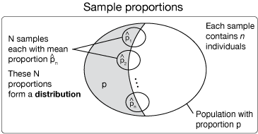
A sample proportion (\(\hat{p}\)) is the fraction of individuals in a sample that have a certain characteristic.  It is calculated as:

\( \hat{p} = \dfrac{\text{number with characteristic}}{\text{sample size } n} \)

The sample proportion is used to estimate the true population proportion \(p\).

Sampling Distributions for Sample Proportions

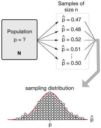
The sampling distribution of a sample proportion describes the distribution of \(\hat{p}\) across all possible random samples of the same size. Key properties:

Sampling Distribution of \(\hat{p}\):

The distribution of sample proportions from all possible random samples of size \(n\) from a population with true proportion \(p\).

Mean (Center):

\(\mu_{\hat{p}} = p\). The sample proportion is an unbiased estimator of the population proportion.

Standard Deviation (Spread):

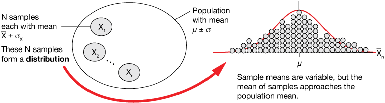
\(\sigma_{\hat{p}} = \sqrt{\dfrac{p(1-p)}{n}}\), provided \(n\) is much smaller than the population size (usually \(n \leq 10\%\) of population).

Shape (Normal Approximation):

The sampling distribution of \(\hat{p}\) is approximately normal if both: \(n \cdot p \geq 10\) and \(n \cdot (1-p) \geq 10\).

Example 

A survey finds that 40% of people in a city prefer online shopping. If a random sample of \( n = 100 \) people is taken:

Find the mean and standard deviation of the sampling distribution of \(\hat{p}\).

▶️ Answer / Explanation

Step 1: Mean: \(\mu_{\hat{p}} = p = 0.40\).

Step 2: Standard Deviation: \(\sigma_{\hat{p}} = \sqrt{\dfrac{0.4(0.6)}{100}} = \sqrt{0.0024} \approx 0.049\).

Answer: The sampling distribution has mean \(0.40\) and standard deviation about \(0.049\).

Example 

Suppose 70% of students at a school support a new policy. A random sample of \( n = 200 \) students is surveyed.

What are the parameters of the sampling distribution of \(\hat{p}\)?

▶️ Answer / Explanation

Step 1: Mean: \(\mu_{\hat{p}} = p = 0.70\).

Step 2: Standard Deviation: \(\sigma_{\hat{p}} = \sqrt{\dfrac{0.7(0.3)}{200}} = \sqrt{0.00105} \approx 0.0324\).

Answer: The sampling distribution has mean \(0.70\) and standard deviation about \(0.032\).

Example 

A population has a true proportion of smokers \( p = 0.25 \). A random sample of \( n = 150 \) people is selected.

Find the mean and standard deviation of the sampling distribution of \(\hat{p}\), and check if normal approximation applies.

▶️ Answer / Explanation

Step 1: Mean: \(\mu_{\hat{p}} = p = 0.25\).

Step 2: Standard Deviation: \(\sigma_{\hat{p}} = \sqrt{\dfrac{0.25(0.75)}{150}} = \sqrt{0.00125} \approx 0.035\).

Step 3: Normal Approximation Check: \(n \cdot p = 150 \cdot 0.25 = 37.5 \geq 10\), and \(n \cdot (1-p) = 112.5 \geq 10\). 

Answer: Mean = \(0.25\), Standard Deviation ≈ \(0.035\), and the distribution is approximately normal.

Normal Approximation for a Sample Proportion

Normal Approximation for a Sample Proportion

The sampling distribution of the sample proportion \(\hat{p}\) is approximately normal if the sample size is large enough.

Rule of Thumb: Both of the following must hold:

    • \( n \cdot p \geq 10 \) (enough expected successes)
    • \( n \cdot (1-p) \geq 10 \) (enough expected failures)

Center: Mean of the sampling distribution is \(\mu_{\hat{p}} = p\).

Spread: Standard deviation is \(\sigma_{\hat{p}} = \sqrt{\dfrac{p(1-p)}{n}}\), provided \(n\) is small compared to the population (usually \(n \leq 10\%\) of population).

Interpretation: If both conditions are met, we can use the normal model to approximate probabilities for sample proportions.

Example

In a city, 30% of households own a dog. A survey samples \( n = 50 \) households.

Can the sampling distribution of \(\hat{p}\) be described as approximately normal?

▶️ Answer / Explanation

Step 1: Compute expected successes: \( n \cdot p = 50 \cdot 0.3 = 15 \geq 10\).

Step 2: Compute expected failures: \( n \cdot (1-p) = 50 \cdot 0.7 = 35 \geq 10\).

Step 3: Both conditions are satisfied.

Answer: Yes, the sampling distribution of \(\hat{p}\) is approximately normal.

Example

A school reports that 8% of students are left-handed. A random sample of \( n = 40 \) students is chosen.

Is the sampling distribution of \(\hat{p}\) approximately normal?

▶️ Answer / Explanation

Step 1: Expected successes: \( n \cdot p = 40 \cdot 0.08 = 3.2 < 10\).

Step 2: Expected failures: \( n \cdot (1-p) = 40 \cdot 0.92 = 36.8 \geq 10\).

Step 3: Since successes < 10, condition is not met.

Answer: No, the sampling distribution cannot be approximated by a normal distribution in this case.

Example

Suppose 55% of voters support a candidate. A random sample of \( n = 120 \) voters is taken.

Check if the sampling distribution of \(\hat{p}\) is approximately normal.

▶️ Answer / Explanation

Step 1: Expected successes: \( n \cdot p = 120 \cdot 0.55 = 66 \geq 10\).

Step 2: Expected failures: \( n \cdot (1-p) = 120 \cdot 0.45 = 54 \geq 10\).

Step 3: Both conditions are satisfied.

Answer: Yes, the sampling distribution is approximately normal.

Interpreting a Sampling Distribution for a Sample Proportion

Interpreting a Sampling Distribution for a Sample Proportion

Mean (Center): \(\mu_{\hat{p}} = p\). The mean of the sampling distribution is equal to the true population proportion. This shows that \(\hat{p}\) is an unbiased estimator of \(p\).

Standard Deviation (Spread): \(\sigma_{\hat{p}} = \sqrt{\dfrac{p(1-p)}{n}}\), which measures how much the sample proportion typically varies from the population proportion.

Normal Approximation: If \(n \cdot p \geq 10\) and \(n \cdot (1-p) \geq 10\), the sampling distribution of \(\hat{p}\) is approximately normal.

Interpretation: Probabilities and parameters must always be described in the context of the population. For example, “There is a 95% probability that the sample proportion of voters in favor will be between 0.46 and 0.54.”

Example 

Suppose 40% of all residents in a city support building a new park (\( p = 0.40 \)). A random sample of \( n = 100 \) residents is taken.

Find and interpret the mean and standard deviation of the sampling distribution of \(\hat{p}\).

▶️ Answer / Explanation

Step 1: Mean: \(\mu_{\hat{p}} = p = 0.40\).

Step 2: Standard Deviation: \(\sigma_{\hat{p}} = \sqrt{\dfrac{0.4(0.6)}{100}} = \sqrt{0.0024} \approx 0.049\).

Step 3 (Interpretation): On average, the sample proportion will equal the true proportion (40%). The sample proportion typically varies about 4.9 percentage points from 40% in repeated samples of size 100.

Example 

A population has a true proportion of smokers \( p = 0.25 \). A random sample of \( n = 150 \) people is chosen.

Interpret the probability that the sample proportion \(\hat{p}\) falls between 0.20 and 0.30.

▶️ Answer / Explanation

Step 1: Parameters: \(\mu_{\hat{p}} = 0.25\), \(\sigma_{\hat{p}} = \sqrt{\dfrac{0.25(0.75)}{150}} = \sqrt{0.00125} \approx 0.035\).

Step 2: Standardize using z-scores: For 0.20: \( z = \dfrac{0.20 – 0.25}{0.035} \approx -1.43 \). For 0.30: \( z = \dfrac{0.30 – 0.25}{0.035} \approx 1.43 \).

Step 3: Probability: \( P(0.20 \leq \hat{p} \leq 0.30) \approx P(-1.43 \leq Z \leq 1.43) \approx 0.846 \).

Interpretation: There is about an 84.6% chance that the sample proportion of smokers will be between 20% and 30% in a random sample of 150 people.

Example 

In a large population, 55% of voters support a policy (\( p = 0.55 \)). If a poll samples \( n = 200 \) voters:

Interpret the sampling distribution of \(\hat{p}\).

▶️ Answer / Explanation

Step 1: Mean: \(\mu_{\hat{p}} = 0.55\).

Step 2: Standard Deviation: \(\sigma_{\hat{p}} = \sqrt{\dfrac{0.55(0.45)}{200}} = \sqrt{0.0012375} \approx 0.035\).

Step 3 (Interpretation): In repeated random samples of 200 voters, the sample proportion of those supporting the policy will center at 55% and typically vary by about 3.5 percentage points. This allows us to make probability statements about possible sample outcomes.

Scroll to Top