Home / AP Statistics 5.6 Sampling Distributions for Differences in Sample Proportions Study Notes

AP Statistics 5.6 Sampling Distributions for Differences in Sample Proportions Study Notes

AP Statistics 5.6 Sampling Distributions for Differences in Sample Proportions Study Notes- New syllabus

AP Statistics 5.6 Sampling Distributions for Differences in Sample Proportions Study Notes -As per latest AP Statistics Syllabus.

LEARNING OBJECTIVE

  • Probabilistic reasoning allows us to anticipate patterns in data

Key Concepts:

  • Sampling Distribution for the Difference in Sample Proportions
  • Normal Approximation for the Difference in Sample Proportions
  • Interpreting a Sampling Distribution for a Difference in Proportions 

AP Statistics -Concise Summary Notes- All Topics

Sampling Distribution for the Difference in Sample Proportions

Sampling Distribution for the Difference in Sample Proportions

 The sampling distribution of \(\hat{p}_1 – \hat{p}_2\) is the distribution of differences between two independent sample proportions from two populations.

Mean (Center):

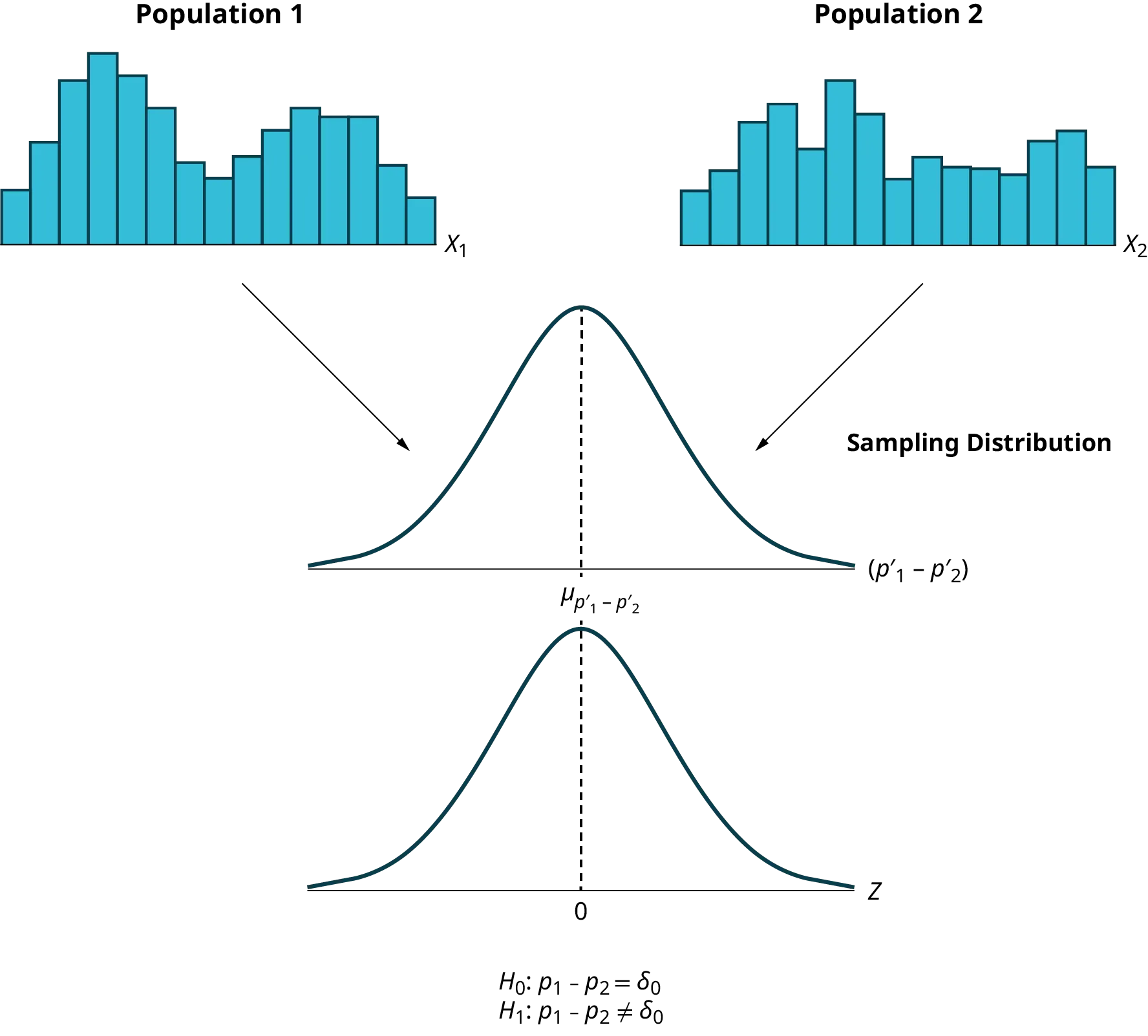
\( \mu_{\hat{p}_1 – \hat{p}_2} = p_1 – p_2 \)

The mean equals the difference in the true population proportions.

Standard Deviation (Spread):

\( \sigma_{\hat{p}_1 – \hat{p}_2} = \sqrt{\dfrac{p_1(1-p_1)}{n_1} + \dfrac{p_2(1-p_2)}{n_2}} \)

Measures how much the difference in sample proportions typically varies from the true difference.

Shape (Normal Approximation): Approximately normal if both samples are independent and for each sample:

\( n_1 \cdot p_1 \geq 10, \quad n_1 \cdot (1-p_1) \geq 10, \quad n_2 \cdot p_2 \geq 10, \quad n_2 \cdot (1-p_2) \geq 10 \)

Interpretation: Probabilities and parameters should be described in the context of the populations.

For example, “The expected difference in sample proportions between group 1 and group 2 is …, with typical variability of ….”

Example 

In a survey, 60% of adults in City A support a new policy (\(p_1 = 0.60\)), and 50% of adults in City B support it (\(p_2 = 0.50\)). A random sample of \(n_1 = 100\) adults from City A and \(n_2 = 120\) adults from City B is taken.

Find the mean and standard deviation of the sampling distribution of \(\hat{p}_1 – \hat{p}_2\).

▶️ Answer / Explanation

Step 1: Mean: \(\mu_{\hat{p}_1 – \hat{p}_2} = p_1 – p_2 = 0.60 – 0.50 = 0.10\).

Step 2: Standard deviation: \(\sigma_{\hat{p}_1 – \hat{p}_2} = \sqrt{\dfrac{0.6(0.4)}{100} + \dfrac{0.5(0.5)}{120}} = \sqrt{0.0024 + 0.0020833} = \sqrt{0.0044833} \approx 0.067\).

Step 3 (Interpretation): On average, the difference in sample proportions is expected to be 0.10, with typical variability about 0.067.

Example 

A study finds that 30% of women (\(p_1 = 0.30\)) and 20% of men (\(p_2 = 0.20\)) in a community exercise regularly. Random samples of \(n_1 = 80\) women and \(n_2 = 70\) men are surveyed.

Determine the mean and standard deviation of the sampling distribution of \(\hat{p}_1 – \hat{p}_2\), and check if normal approximation applies.

▶️ Answer / Explanation

Step 1: Mean: \(\mu_{\hat{p}_1 – \hat{p}_2} = 0.30 – 0.20 = 0.10\).

Step 2: Standard deviation: \(\sigma_{\hat{p}_1 – \hat{p}_2} = \sqrt{\dfrac{0.3(0.7)}{80} + \dfrac{0.2(0.8)}{70}} = \sqrt{0.002625 + 0.002286} = \sqrt{0.004911} \approx 0.070\).

Step 3: Normal approximation check: \( n_1 \cdot p_1 = 80 \cdot 0.3 = 24 \geq 10\), \( n_1 \cdot (1-p_1) = 80 \cdot 0.7 = 56 \geq 10\), \( n_2 \cdot p_2 = 70 \cdot 0.2 = 14 \geq 10\), \( n_2 \cdot (1-p_2) = 70 \cdot 0.8 = 56 \geq 10 \)

Step 4 (Interpretation): The expected difference in sample proportions is 0.10, with typical variability of about 0.070, and the distribution is approximately normal.

Normal Approximation for the Difference in Sample Proportions

Normal Approximation for the Difference in Sample Proportions

The sampling distribution of \(\hat{p}_1 – \hat{p}_2\) can be approximated as normal if both samples are independent and each sample has sufficiently many expected successes and failures.

Rule of Thumb (Normal Approximation Conditions):

  • Sample 1: \( n_1 \cdot p_1 \geq 10 \) and \( n_1 \cdot (1-p_1) \geq 10 \)
  • Sample 2: \( n_2 \cdot p_2 \geq 10 \) and \( n_2 \cdot (1-p_2) \geq 10 \)

Interpretation: If all four conditions are satisfied, the sampling distribution of \(\hat{p}_1 – \hat{p}_2\) is approximately normal. This allows the use of z-scores and normal probability calculations to analyze differences in sample proportions.

Example 

In two cities, 55% of adults in City A (\(p_1 = 0.55\)) and 45% of adults in City B (\(p_2 = 0.45\)) support a new policy.

Random samples: \(n_1 = 100\), \(n_2 = 120\).

 Can the sampling distribution of \(\hat{p}_1 – \hat{p}_2\) be approximated as normal?

▶️ Answer / Explanation

Step 1: Check expected successes and failures:

  • Sample 1: \(100 \cdot 0.55 = 55 \geq 10\), \(100 \cdot 0.45 = 45 \geq 10\)
  • Sample 2: \(120 \cdot 0.45 = 54 \geq 10\), \(120 \cdot 0.55 = 66 \geq 10\)

Step 2: All conditions satisfied.

Answer: Yes, the sampling distribution is approximately normal.

Example 

In two schools, 8% of students in School A (\(p_1 = 0.08\)) and 12% in School B (\(p_2 = 0.12\)) participate in a special program.

Random samples: \(n_1 = 30\), \(n_2 = 25\).

Can the sampling distribution of \(\hat{p}_1 – \hat{p}_2\) be approximated as normal?

▶️ Answer / Explanation

Step 1: Check expected successes and failures:

  • Sample 1: \(30 \cdot 0.08 = 2.4 < 10\), \(30 \cdot 0.92 = 27.6 \geq 10\)
  • Sample 2: \(25 \cdot 0.12 = 3 < 10\), \(25 \cdot 0.88 = 22 \geq 10\)

Step 2: Some conditions not satisfied.

Answer: No, the sampling distribution cannot be approximated as normal.

Interpreting a Sampling Distribution for a Difference in Proportions 

Interpreting a Sampling Distribution for a Difference in Proportions 

Mean (Center):

\(\mu_{\hat{p}_1 – \hat{p}_2} = p_1 – p_2\).

The expected difference in sample proportions equals the true difference in population proportions.

Standard Deviation (Spread):

\(\sigma_{\hat{p}_1 – \hat{p}_2} = \sqrt{\dfrac{p_1(1-p_1)}{n_1} + \dfrac{p_2(1-p_2)}{n_2}}\).

Measures typical variation of the difference between sample proportions from the true difference.

Probabilities: If approximately normal, probabilities describe the likelihood that the observed difference in sample proportions falls within a certain range.

Context: Always interpret probabilities and parameters in terms of the specific populations being studied. For example: “There is approximately a $95\%$ chance that the difference in sample proportions of voters supporting a policy will be between 0.02 and 0.18.”

Example

In a study, 60% of adults in City A (\(p_1 = 0.60\)) and 50% of adults in City B (\(p_2 = 0.50\)) support a new policy. Random samples: \(n_1 = 100\) from City A, \(n_2 = 120\) from City B.

Interpret the mean, standard deviation, and probability that the difference in sample proportions (\(\hat{p}_1 – \hat{p}_2\)) is between 0.02 and 0.18.

▶️ Answer / Explanation

Step 1: Mean (Expected Difference)

\(\mu_{\hat{p}_1 – \hat{p}_2} = p_1 – p_2 = 0.60 – 0.50 = 0.10\)

Step 2: Standard Deviation

\(\sigma_{\hat{p}_1 – \hat{p}_2} = \sqrt{\dfrac{0.6(0.4)}{100} + \dfrac{0.5(0.5)}{120}} = \sqrt{0.0024 + 0.002083} = \sqrt{0.004483} \approx 0.067\)

Step 3: Probability using Normal Approximation Standardize the interval:

\( z_1 = \frac{0.02 – 0.10}{0.067} \approx -1.19, \quad z_2 = \frac{0.18 – 0.10}{0.067} \approx 1.19 \)

Probability: \( P(0.02 \leq \hat{p}_1 – \hat{p}_2 \leq 0.18) \approx P(-1.19 \leq Z \leq 1.19) \approx 0.882 \)

Step 4: Interpretation There is approximately an 88.2% chance that the observed difference in sample proportions will fall between 0.02 and 0.18. The mean difference is 0.10, with typical variability of about 0.067.

Scroll to Top