Determine Parameters for a Sampling Distribution for Sample Means
Definition of Sample Mean: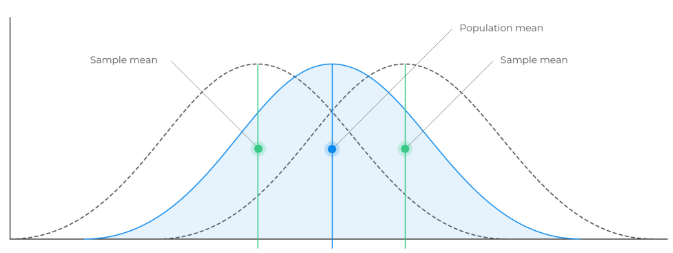
The sample mean, denoted by \( \bar{x} \), is the average of the values in a sample of size \( n \):
\( \bar{x} = \dfrac{\sum_{i=1}^{n} x_i}{n} \)
It is used as an estimator of the population mean \( \mu \).
Mean of the Sampling Distribution:
The mean of the sampling distribution of sample means is equal to the population mean:
\( \mu_{\bar{x}} = \mu \)
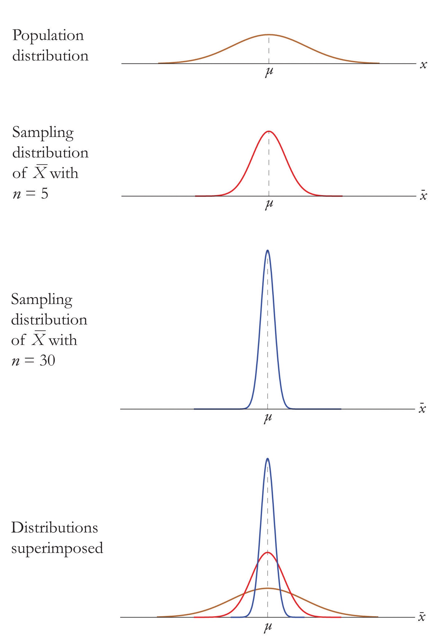
Standard Deviation (Standard Error):
The standard deviation of the sampling distribution (called the standard error) is:
\( \sigma_{\bar{x}} = \dfrac{\sigma}{\sqrt{n}} \) where \( \sigma \) is the population standard deviation and \( n \) is the sample size.
Shape of the Distribution:
If the population is normal, then the sampling distribution of \(\bar{x}\) is normal for any sample size.
If the population is not normal, the sampling distribution of \(\bar{x}\) becomes approximately normal if \( n \) is sufficiently large (Central Limit Theorem).
Example
A population of test scores has mean \( \mu = 80 \) and standard deviation \( \sigma = 12 \). A sample of size \( n = 36 \) is taken.
Find
- The mean of the sampling distribution of sample means.
- The standard deviation (standard error).
▶️ Answer / Explanation
Step 1: Mean of the sampling distribution
\( \mu_{\bar{x}} = \mu = 80 \)
Step 2: Standard error
\( \sigma_{\bar{x}} = \dfrac{\sigma}{\sqrt{n}} = \dfrac{12}{\sqrt{36}} = \dfrac{12}{6} = 2 \)
Answer: \( \mu_{\bar{x}} = 80 \), \( \sigma_{\bar{x}} = 2 \).
Example
A population of household incomes has mean \( \mu = 50{,}000 \) and standard deviation \( \sigma = 15{,}000 \). The population distribution is right-skewed. Suppose we take a random sample of \( n = 100 \) households.
Find:
- The mean of the sampling distribution of sample means.
- The standard error.
- The approximate shape of the distribution of \( \bar{x} \).
▶️ Answer / Explanation
Step 1: Mean of the sampling distribution
\( \mu_{\bar{x}} = \mu = 50{,}000 \)
Step 2: Standard error
\( \sigma_{\bar{x}} = \dfrac{\sigma}{\sqrt{n}} = \dfrac{15{,}000}{\sqrt{100}} = \dfrac{15{,}000}{10} = 1{,}500 \)
Step 3: Shape
Although the population is skewed, by the Central Limit Theorem, the sampling distribution of \( \bar{x} \) is approximately normal because \( n = 100 \) is large.
Answer: \( \mu_{\bar{x}} = 50{,}000 \), \( \sigma_{\bar{x}} = 1{,}500 \), distribution ≈ normal.
Determine Whether a Sampling Distribution of a Sample Mean is Approximately Normal
The sampling distribution of the sample mean \( \bar{x} \) can often be treated as approximately normal. To decide this, check the following:
- If the population is normal: Then the sampling distribution of \( \bar{x} \) is normal for any sample size \( n \).
- If the population is not normal: Use the Central Limit Theorem (CLT). For sufficiently large \( n \) (commonly \( n \geq 30 \)), the sampling distribution of \( \bar{x} \) will be approximately normal.
- Independence condition: Sample observations should be independent. This is generally true if sampling is random and the sample size is no more than 10% of the population.
Summary: The sampling distribution of \( \bar{x} \) is approximately normal if the population itself is normal or if the sample size is large enough (by CLT).
Example :
A population of exam scores is normally distributed with mean \( \mu = 70 \) and standard deviation \( \sigma = 10 \). A sample of size \( n = 15 \) is taken.
Can the sampling distribution of \( \bar{x} \) be described as approximately normal?
▶️ Answer / Explanation
Step 1: Population distribution
The population is normal.
Step 2: Rule
If the population is normal, then the sampling distribution of \( \bar{x} \) is normal for any \( n \).
Answer: Yes, the sampling distribution is normal because the population itself is normal.
Example :
A population of household incomes is right-skewed with mean \( \mu = 60{,}000 \) and standard deviation \( \sigma = 20{,}000 \). A random sample of size \( n = 50 \) is taken.
Can the sampling distribution of \( \bar{x} \) be described as approximately normal?
▶️ Answer / Explanation
Step 1: Population distribution
The population is right-skewed, not normal.
Step 2: Central Limit Theorem
Since \( n = 50 \) (large sample), CLT applies. Thus, the sampling distribution of \( \bar{x} \) is approximately normal.
Answer: Yes, the sampling distribution is approximately normal because the sample size is large enough for CLT.