Determine Parameters of a Sampling Distribution for a Difference in Sample Means
Statistic of interest: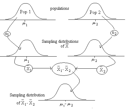
The difference between two independent sample means, \( \bar{x}_1 – \bar{x}_2 \).
Mean of the sampling distribution:
\( \mu_{\bar{x}_1 – \bar{x}_2} = \mu_1 – \mu_2 \)
Interpretation: On average, the difference between sample means equals the difference between the population means.
Standard error of the sampling distribution:
\( \sigma_{\bar{x}_1 – \bar{x}_2} = \sqrt{\dfrac{\sigma_1^2}{n_1} + \dfrac{\sigma_2^2}{n_2}} \) where \( \sigma_1, \sigma_2 \) are the population standard deviations, and \( n_1, n_2 \) are the sample sizes.
Shape: If both populations are normal, the distribution of \( \bar{x}_1 – \bar{x}_2 \) is normal. If not, the Central Limit Theorem ensures approximate normality when \( n_1 \) and \( n_2 \) are sufficiently large.
Conditions: Samples must be independent, and each sample should be random. For finite populations, the sample size should not exceed $10\%$ of the population size.
Example:
A researcher compares the average test scores of two schools.
School A population: \( \mu_1 = 75 \), \( \sigma_1 = 10 \), sample size \( n_1 = 40 \).
School B population: \( \mu_2 = 70 \), \( \sigma_2 = 12 \), sample size \( n_2 = 50 \).
Find the mean and standard error of the sampling distribution of \( \bar{x}_1 – \bar{x}_2 \).
▶️ Answer / Explanation
Step 1: Mean
\( \mu_{\bar{x}_1 – \bar{x}_2} = \mu_1 – \mu_2 = 75 – 70 = 5 \).
Interpretation: On average, School A’s sample mean score is 5 points higher than School B’s.
Step 2: Standard Error
\( \sigma_{\bar{x}_1 – \bar{x}_2} = \sqrt{\dfrac{\sigma_1^2}{n_1} + \dfrac{\sigma_2^2}{n_2}} = \sqrt{\dfrac{10^2}{40} + \dfrac{12^2}{50}} \).
\( = \sqrt{\dfrac{100}{40} + \dfrac{144}{50}} = \sqrt{2.5 + 2.88} = \sqrt{5.38} \approx 2.32 \).
Final Answer: Mean = 5, Standard Error ≈ 2.32.
Example
A nutritionist studies the average daily calorie intake of two groups.
Group 1: \( \mu_1 = 2200 \), \( \sigma_1 = 400 \), sample size \( n_1 = 64 \).
Group 2: \( \mu_2 = 2100 \), \( \sigma_2 = 500 \), sample size \( n_2 = 100 \).
Find the mean and standard error of the sampling distribution of \( \bar{x}_1 – \bar{x}_2 \).
▶️ Answer / Explanation
Step 1: Mean
\( \mu_{\bar{x}_1 – \bar{x}_2} = 2200 – 2100 = 100 \).
Interpretation: On average, Group 1 consumes 100 more calories per day than Group 2.
Step 2: Standard Error
\( \sigma_{\bar{x}_1 – \bar{x}_2} = \sqrt{\dfrac{400^2}{64} + \dfrac{500^2}{100}} \).
\( = \sqrt{\dfrac{160000}{64} + \dfrac{250000}{100}} = \sqrt{2500 + 2500} = \sqrt{5000} \approx 70.71 \).
Final Answer: Mean = 100, Standard Error ≈ 70.71.
Approximate Normality for $\bar{x}_1 – \bar{x}_2$
If both populations are normal Then the sampling distribution of \( \bar{x}_1 – \bar{x}_2 \) is normal, regardless of sample sizes.
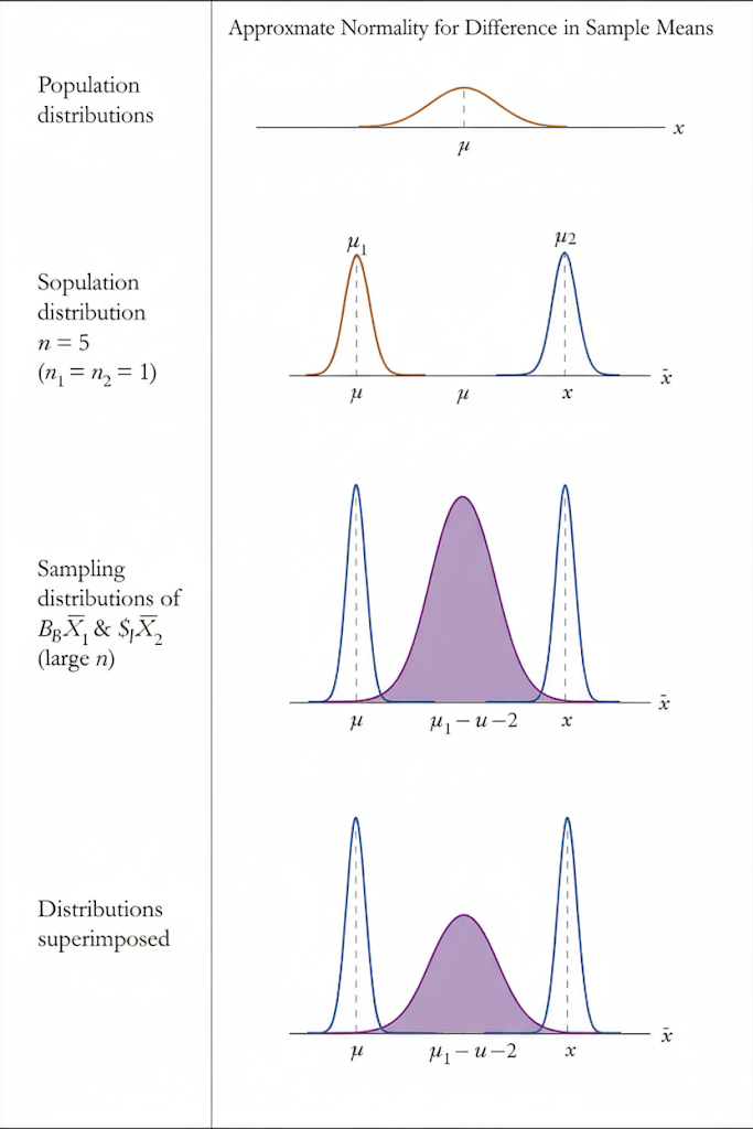
- If populations are not normal: By the Central Limit Theorem (CLT), the sampling distribution of \( \bar{x}_1 – \bar{x}_2 \) will be approximately normal if both sample sizes are sufficiently large (commonly \( n_1, n_2 \geq 30 \)).
- Independence condition: The two samples must be independent. If sampling without replacement, sample sizes should be no more than 10% of the population sizes.
Approximate normality depends on (1) shape of population distributions and (2) size of samples.
Example:
Researchers compare average study times of two groups of students.
- Group 1: population not normal, \( n_1 = 40 \).
- Group 2: population not normal, \( n_2 = 35 \).
Can the sampling distribution of \( \bar{x}_1 – \bar{x}_2 \) be treated as approximately normal?
▶️ Answer / Explanation
Step 1: Populations are not normal. So we must use the CLT.
Step 2: Both sample sizes are large enough (\( n_1 = 40 \), \( n_2 = 35 \), both ≥ 30).
Step 3: Samples are independent (assumed random and from different groups).
Conclusion: By the Central Limit Theorem, the sampling distribution of \( \bar{x}_1 – \bar{x}_2 \) can be described as approximately normal.