Home / AP Statistics 6.10 Setting Up a Test for the Difference of Two Population Proportions Study Notes

AP Statistics 6.10 Setting Up a Test for the Difference of Two Population Proportions Study Notes

AP Statistics 6.10 Setting Up a Test for the Difference of Two Population Proportions Study Notes- New syllabus

AP Statistics 6.10 Setting Up a Test for the Difference of Two Population Proportions Study Notes -As per latest AP Statistics Syllabus.

LEARNING OBJECTIVE

  • The normal distribution may be used to model variation.

Key Concepts:

  • Null and Alternative Hypotheses for a Difference of Two Population Proportions
  • Testing the Difference of Two Population Proportions
  • Conditions for Testing a Difference of Two Population Proportions

AP Statistics -Concise Summary Notes- All Topics

Null and Alternative Hypotheses for a Difference of Two Population Proportions

Null and Alternative Hypotheses for a Difference of Two Population Proportions

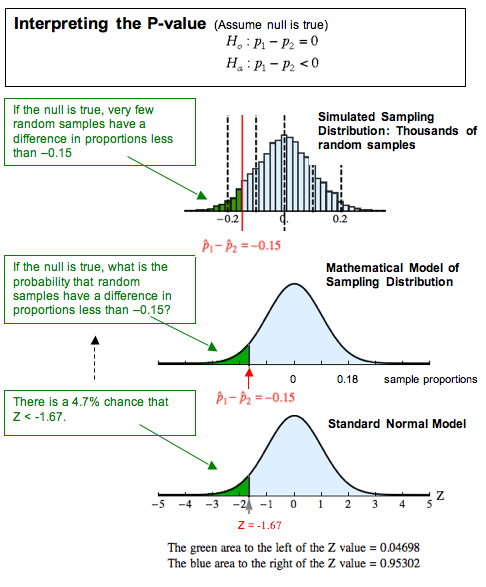
When testing for a difference between two population proportions, we are interested in comparing:

\( p_1 \) = population proportion for group 1

\( p_2 \) = population proportion for group 2

General Null Hypothesis (\( H_0 \)):

\( H_0: p_1 – p_2 = 0 \)    or equivalently    \( H_0: p_1 = p_2 \)

This states that there is no difference between the population proportions.

Alternative Hypotheses (\( H_a \)):

  • Two-sided test: \( H_a: p_1 – p_2 \neq 0 \) (There is a difference between the two population proportions.)
  • One-sided test (greater than): \( H_a: p_1 – p_2 > 0 \) (The population proportion in group 1 is greater than in group 2.)
  • One-sided test (less than): \( H_a: p_1 – p_2 < 0 \) (The population proportion in group 1 is less than in group 2.)

Key Notes:

  • The null hypothesis always assumes no difference between the two population proportions.
  • The choice of a one-sided or two-sided alternative depends on the context of the research question.
  • Always define \( p_1 \) and \( p_2 \) clearly in context before writing hypotheses.

Example:

A survey asks whether high school students and college students prefer online classes. The data collected shows:

  • Group 1 (High School): sample proportion \( \hat{p}_1 = 0.55 \), sample size \( n_1 = 120 \)
  • Group 2 (College): sample proportion \( \hat{p}_2 = 0.48 \), sample size \( n_2 = 150 \)

State the null and alternative hypotheses for testing whether there is a difference in the true proportions of students who prefer online classes.

▶️ Answer / Explanation

Step 1: Define parameters: \( p_1 \) = true proportion of high school students who prefer online classes \( p_2 \) = true proportion of college students who prefer online classes

Step 2: State hypotheses:

  • Null hypothesis: \( H_0: p_1 – p_2 = 0 \) (no difference in the population proportions)
  • Alternative hypothesis: \( H_a: p_1 – p_2 \neq 0 \) (there is a difference in the population proportions)

Step 3: This is a two-sided test since the question is asking whether the proportions are different, without specifying which group is higher.

Testing the Difference of Two Population Proportions

Testing the Difference of Two Population Proportions

When comparing two population proportions, the appropriate testing method is the two-sample z-test for proportions. This test evaluates whether there is a statistically significant difference between two population proportions \( p_1 \) and \( p_2 \).

Step 1: Identify Parameters

  • \( p_1 \) = population proportion for group 1
  • \( p_2 \) = population proportion for group 2

Step 2: State Hypotheses

  • Null Hypothesis (\( H_0 \)): \( p_1 – p_2 = 0 \) (no difference between population proportions)
  • Alternative Hypothesis (\( H_a \)):
    • Two-sided: \( p_1 – p_2 \neq 0 \)
    • One-sided (greater): \( p_1 – p_2 > 0 \)
    • One-sided (less): \( p_1 – p_2 < 0 \)

Step 3: Test Statistic

The test statistic is based on the difference between sample proportions:

\( z = \dfrac{(\hat{p}_1 – \hat{p}_2) – (p_1 – p_2)_{0}}{SE} \)

where under the null hypothesis, \( (p_1 – p_2)_{0} = 0 \).

The standard error is calculated using the pooled proportion (since \( H_0 \) assumes \( p_1 = p_2 \)):

\( \hat{p} = \dfrac{x_1 + x_2}{n_1 + n_2} \)

\( SE = \sqrt{\hat{p}(1 – \hat{p})\left(\dfrac{1}{n_1} + \dfrac{1}{n_2}\right)} \)

Step 4: Distribution

Assuming the conditions are met, the test statistic follows a standard Normal distribution (\( z \)).

Step 5: Decision Rule

  • Calculate the p-value based on the \( z \)-statistic and the alternative hypothesis form.
  • Compare the p-value to the chosen significance level (\( \alpha \)).
  • If \( p\text{-value} \leq \alpha \), reject \( H_0 \); otherwise, fail to reject \( H_0 \).

Example :

A researcher wants to know whether the proportion of customers who prefer Brand A differs between two cities. A random sample yields:

  • City 1: \(x_1 = 90\) out of \(n_1 = 150\) prefer Brand A (\(\hat{p}_1 = 0.60\)).
  • City 2: \(x_2 = 110\) out of \(n_2 = 200\) prefer Brand A (\(\hat{p}_2 = 0.55\)).

Test at the \(\alpha=0.05\) level whether the population proportions differ.

▶️ Answer / Explanation

Step 1: State the hypotheses

\( H_0: p_1 – p_2 = 0 \) (no difference)
\( H_a: p_1 – p_2 \neq 0 \) (two-sided)

Step 2: Verify conditions

  • Random samples: assumed. 
  • Independence: samples from distinct cities, and \(n_1 \le 0.1N_1,\; n_2 \le 0.1N_2\) assumed. 
  • Large counts: \(n_1\hat{p}_1 = 150(0.60)=90\), \(n_1(1-\hat{p}_1)=60\); \(n_2\hat{p}_2=200(0.55)=110\), \(n_2(1-\hat{p}_2)=90\). All ≥ 10. 

Step 3: Compute pooled proportion and standard error

Under \(H_0\) assume \(p_1=p_2=p\). The pooled estimate is \(\displaystyle \hat{p}=\dfrac{x_1+x_2}{n_1+n_2}=\dfrac{90+110}{150+200}= \dfrac{200}{350}\approx 0.5714.\)

Standard error for the difference (using pooled \( \hat{p} \)): \(\displaystyle SE=\sqrt{\hat{p}(1-\hat{p})\left(\dfrac{1}{n_1}+\dfrac{1}{n_2}\right)} =\sqrt{0.5714(0.4286)\left(\dfrac{1}{150}+\dfrac{1}{200}\right)}\approx 0.05345.\)

Step 4: Test statistic

\(\displaystyle z=\dfrac{\hat{p}_1-\hat{p}_2}{SE}=\dfrac{0.60-0.55}{0.05345}\approx 0.9354.\)

Step 5: P-value (two-sided)

Two-tailed p-value = \(2\cdot P(Z>|0.9354|)\approx 0.35.\)

Step 6: Decision

Since p-value ≈ \(0.35 > \alpha=0.05\), we fail to reject \(H_0\).

Conclusion (in context): There is insufficient statistical evidence at the 5% level to conclude that the proportion of customers who prefer Brand A differs between City 1 and City 2.

Conditions for Testing a Difference of Two Population Proportions

Conditions for Testing a Difference of Two Population Proportions

When conducting a two-sample z-test for proportions, the following conditions must be verified:

1. Random:

  • Data should come from two independent random samples or from a randomized experiment.

2. Independence:

  • Each sample must represent less than 10% of its population when sampling without replacement.
    Check: \( n_1 \leq 0.1N_1 \) and \( n_2 \leq 0.1N_2 \).
  • The two samples must also be independent of each other.

3. Normal (Large Counts Condition):

  • To check that the sampling distribution of \( \hat{p}_1 – \hat{p}_2 \) is approximately Normal, we use the combined (or pooled) proportion under the null hypothesis \( H_0: p_1 = p_2 \).

The pooled proportion is defined as:

\(\displaystyle \hat{p} = \dfrac{x_1 + x_2}{n_1 + n_2}\)

Then check expected counts for both groups using \( \hat{p} \):

  • \( n_1\hat{p} \geq 10 \) and \( n_1(1 – \hat{p}) \geq 10 \)
  • \( n_2\hat{p} \geq 10 \) and \( n_2(1 – \hat{p}) \geq 10 \)

If all four conditions are met, the distribution of \( \hat{p}_1 – \hat{p}_2 \) can be approximated by a Normal model.

Example 

A researcher compares the proportion of adults who exercise regularly in two cities. A random survey yields:

  • City 1: \(x_1 = 78\) successes out of \(n_1 = 120\).
  • City 2: \(x_2 = 88\) successes out of \(n_2 = 150\).

Verify whether the conditions for performing a two-sample z-test for \(p_1 – p_2\) are satisfied.

▶️ Answer / Explanation

Step 1 — Random:

The problem states these are random surveys. We assume each sample was collected randomly or via a randomized procedure. Random condition: satisfied.

Step 2 — Independence (including 10% condition):

  • The two samples come from different cities, so they are independent of each other. Independence between samples: satisfied.
  • For sampling without replacement we require each sample to be ≤ 10% of its population: \(n_1 \le 0.1N_1\) and \(n_2 \le 0.1N_2\).
    Assuming each city’s adult population is much larger than 120 and 150, the 10% condition is likely satisfied. 10% condition: satisfied (assumed).

Step 3 — Normal (large counts) using pooled proportion under \(H_0\):

For hypothesis testing we check large counts with the pooled proportion under \(H_0\):

\(\displaystyle \hat{p}=\dfrac{x_1+x_2}{n_1+n_2}=\dfrac{78+88}{120+150}=\dfrac{166}{270}\approx 0.615.\)

Now check expected successes and failures in each sample using \(\hat{p}\):

  • City 1 successes: \(n_1\hat{p}=120(0.615)\approx 73.8 \ge 10\).
  • City 1 failures: \(n_1(1-\hat{p})=120(0.385)\approx 46.2 \ge 10\).
  • City 2 successes: \(n_2\hat{p}=150(0.615)\approx 92.3 \ge 10\).
  • City 2 failures: \(n_2(1-\hat{p})=150(0.385)\approx 57.8 \ge 10\).

All four counts are at least 10, so the sampling distribution of \(\hat{p}_1-\hat{p}_2\) can be approximated by a Normal distribution. Normal (large counts) condition: satisfied.

Conclusion:

All required conditions — random sampling, independence (including the 10% condition), and the large counts condition using the pooled proportion — are satisfied. It is appropriate to proceed with a two-sample z-test for the difference in population proportions \(p_1 – p_2\).

Scroll to Top