Home / AP Statistics 6.11 Carrying Out a Test for the Difference of Two Population Proportions Study Notes

AP Statistics 6.11 Carrying Out a Test for the Difference of Two Population Proportions Study Notes

AP Statistics 6.11 Carrying Out a Test for the Difference of Two Population Proportions Study Notes- New syllabus

AP Statistics 6.11 Carrying Out a Test for the Difference of Two Population Proportions Study Notes -As per latest AP Statistics Syllabus.

LEARNING OBJECTIVE

  • The normal distribution may be used to model variation.

Key Concepts:

  • Test Statistic for the Difference of Two Population Proportions
  • Interpret the p-value of a Significance Test for a Difference of Two Population Proportions
  • Justifying a Claim Based on a Significance Test for a Difference of Two Population Proportions

AP Statistics -Concise Summary Notes- All Topics

Test Statistic for the Difference of Two Population Proportions

Test Statistic for the Difference of Two Population Proportions

We use a two-sample z-test for proportions to test hypotheses about \( p_1 – p_2 \).

Step 1: Define the test statistic

The test statistic measures how far the observed difference in sample proportions is from the null hypothesis difference (usually 0), in terms of standard errors:

\(\displaystyle z = \dfrac{(\hat{p}_1 – \hat{p}_2) – (p_1 – p_2)_0}{SE}\)

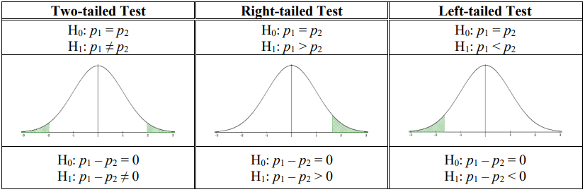
  • \(\hat{p}_1 = \dfrac{x_1}{n_1}\), \(\hat{p}_2 = \dfrac{x_2}{n_2}\)
  • \((p_1 – p_2)_0\) = hypothesized difference (most often 0)

Step 2: Standard Error using Pooled Proportion

When the null hypothesis states \(p_1 = p_2\), we use the pooled proportion:

\(\displaystyle \hat{p} = \dfrac{x_1 + x_2}{n_1 + n_2}\)

The standard error is:

\(\displaystyle SE = \sqrt{\hat{p}(1 – \hat{p})\left(\dfrac{1}{n_1} + \dfrac{1}{n_2}\right)}\)

Step 3: Distribution

Under the null hypothesis, the test statistic follows a standard Normal distribution (\(z\)).

Test Statistic for the Difference of Two Population Proportions

The test statistic is:

\(\displaystyle z = \dfrac{(\hat{p}_1 – \hat{p}_2) – 0}{\sqrt{\hat{p}_c(1 – \hat{p}_c)\left(\dfrac{1}{n_1} + \dfrac{1}{n_2}\right)}}\)

where the pooled proportion is defined as:

\(\displaystyle \hat{p}_c = \dfrac{n_1\hat{p}_1 + n_2\hat{p}_2}{n_1 + n_2}\)

Example

A researcher studies whether there is a difference in support for a new policy between two towns:

  • Town 1: \(x_1 = 56\) out of \(n_1 = 100\) support the policy (\(\hat{p}_1 = 0.56\))
  • Town 2: \(x_2 = 63\) out of \(n_2 = 120\) support the policy (\(\hat{p}_2 = 0.525\))

 Calculate the test statistic for testing \(H_0: p_1 = p_2\).

▶️ Answer / Explanation

Step 1: Define hypotheses

\(H_0: p_1 – p_2 = 0\) \(H_a: p_1 – p_2 \neq 0\) (two-sided)

Step 2: Calculate pooled proportion

\(\displaystyle \hat{p} = \dfrac{x_1 + x_2}{n_1 + n_2} = \dfrac{56 + 63}{100 + 120} = \dfrac{119}{220} \approx 0.541.\)

Step 3: Standard error using pooled \(\hat{p}\)

\(\displaystyle SE = \sqrt{\hat{p}(1-\hat{p})\left(\dfrac{1}{n_1} + \dfrac{1}{n_2}\right)}\)

\(\displaystyle SE = \sqrt{0.541(0.459)\left(\dfrac{1}{100} + \dfrac{1}{120}\right)}\)

\(\displaystyle SE = \sqrt{0.248\left(0.010 + 0.00833\right)} = \sqrt{0.248(0.01833)} \approx \sqrt{0.00455} \approx 0.0675.\)

Step 4: Compute test statistic

\(\displaystyle z = \dfrac{(\hat{p}_1 – \hat{p}_2) – 0}{SE} = \dfrac{0.56 – 0.525}{0.0675} = \dfrac{0.035}{0.0675} \approx 0.52.\)

Final Answer:

The test statistic is \(z \approx 0.52\).

Interpret the p-value of a Significance Test for a Difference of Two Population Proportions

Interpret the p-value of a Significance Test for a Difference of Two Population Proportions

Definition of p-value:

The p-value is the probability of obtaining a test statistic as extreme or more extreme than the observed test statistic, assuming the null hypothesis \(H_0: p_1 = p_2\) is true.

Interpretation based on the alternative hypothesis:

  • If \(H_a: p_1 > p_2\), the p-value is the probability that the null distribution produces a difference at least as large as the observed \(\hat{p}_1 – \hat{p}_2\).
  • If \(H_a: p_1 < p_2\), the p-value is the probability that the null distribution produces a difference at most as small as the observed \(\hat{p}_1 – \hat{p}_2\).
  • If \(H_a: p_1 \neq p_2\), the p-value is the probability that the null distribution produces a difference as extreme or more extreme in either direction than the observed \(\hat{p}_1 – \hat{p}_2\).

Key points:

  • A small p-value suggests the observed difference is unlikely under the null hypothesis, giving evidence for the alternative hypothesis.
  • A large p-value suggests the observed difference is consistent with the null hypothesis, and does not provide convincing evidence for the alternative.
  • The interpretation must always be stated in the context of the populations being compared (not just in statistical terms).

Example of interpretation:

Suppose a test comparing support rates between Town A and Town B gives \(p\text{-value} = 0.04\) for a two-sided test at \(\alpha = 0.05\).

Interpretation: If the true support rates in the two towns are equal, there is only a 4% chance of obtaining a difference in sample proportions as extreme or more extreme than the observed difference. Since 0.04 < 0.05, this provides statistically significant evidence that the population proportions differ.

Example 

A study was conducted to compare the proportion of students who prefer online classes in two schools, School A and School B. Out of 120 students in School A, 72 preferred online classes, while out of 150 students in School B, 75 preferred online classes. A two-sided hypothesis test was conducted, and the p-value was found to be 0.03.

What is the correct interpretation of this p-value?

  1. There is a 3% chance that the true population proportions are equal.
  2. If the true population proportions are equal, there is a 3% chance of observing a sample difference in proportions as extreme or more extreme than the one observed.
  3. The probability that the null hypothesis is true is 0.03.
  4. There is a 97% chance that the alternative hypothesis is true.
▶️ Answer / Explanation

Correct Answer: B

The p-value is not the probability that the null hypothesis is true (A and C are wrong), nor is it the probability the alternative is true (D is wrong).

Instead, it represents the probability of getting a difference in sample proportions as extreme or more extreme than the observed difference, assuming the null hypothesis \(H_0: p_1 = p_2\) is true.

Justifying a Claim Based on a Significance Test for a Difference of Two Population Proportions

Justifying a Claim Based on a Significance Test for a Difference of Two Population Proportions

Step 1: Recall the purpose of the test

A significance test for two population proportions evaluates evidence about whether there is a true difference between the proportions, denoted \( p_1 – p_2 \).

Step 2: Role of significance level

  • The significance level (\( \alpha \)) is the threshold for making a decision. Common choices are 0.05 or 0.01.
  • \( \alpha \) is the probability of making a Type I error (rejecting the null hypothesis when it is true).
  • The smaller the significance level, the stronger the evidence required to reject the null hypothesis.

Step 3: Interpreting the p-value

  • The p-value is the probability of observing a difference in sample proportions as extreme or more extreme than the observed difference, assuming the null hypothesis \( H_0: p_1 = p_2 \) is true.
  • If \( p\text{-value} \leq \alpha \): Reject \( H_0 \). There is sufficient evidence to support the claim that \( p_1 \neq p_2 \) (or \( p_1 > p_2 \), \( p_1 < p_2 \), depending on the alternative).
  • If \( p\text{-value} > \alpha \): Fail to reject \( H_0 \). There is insufficient evidence to support the claim. This does not mean the null is proven true.

Step 4: Drawing a conclusion in context

  • Rejecting the null hypothesis: Suggests that the observed difference in sample proportions is unlikely to have occurred by chance alone. We conclude that there is convincing evidence of a difference in the population proportions.
  • Failing to reject the null hypothesis: Suggests that the sample data do not provide strong enough evidence to conclude that there is a true difference. We cannot rule out that the observed difference is due to sampling variability.

Important notes

  • Rejecting \( H_0 \) does not prove the alternative hypothesis; it only indicates strong evidence against the null.
  • Failing to reject \( H_0 \) does not prove the null hypothesis true; it only means that the evidence was not strong enough to support the alternative.
  • The conclusion must always be stated in the context of the populations being studied.

Example 

A researcher claims that the proportion of voters who support Measure X is higher in City 1 than in City 2. A random survey yields:

  • City 1: \(x_1 = 130\) out of \(n_1 = 200\) support the measure (\(\hat{p}_1 = 0.65\)).
  • City 2: \(x_2 = 150\) out of \(n_2 = 250\) support the measure (\(\hat{p}_2 = 0.60\)).

Claim to test: \(p_1 > p_2\). Use \(\alpha = 0.05\).

▶️ Answer / Explanation

Step 1 — State hypotheses

\(H_0:\; p_1 – p_2 = 0\)
\(H_a:\; p_1 – p_2 > 0\) (one-sided, because the claim is “greater”)

Step 2 — Verify conditions

    • Random: surveys are random (given). 
    • Independence / 10%: samples are from different cities and each sample is assumed < 10% of its city population. 
    • Large counts (use pooled \(\hat{p}\) for test):

Pooled proportion: \(\displaystyle \hat{p}=\dfrac{x_1+x_2}{n_1+n_2}=\dfrac{130+150}{200+250}=\dfrac{280}{450}\approx 0.6222.\)

Check counts: \(n_1\hat{p}=200(0.6222)\approx124.4\), \(n_1(1-\hat{p})\approx75.6\); \(n_2\hat{p}=250(0.6222)\approx155.6\), \(n_2(1-\hat{p})\approx94.4\). All ≥ 10. 

Step 3 — Compute test statistic

Standard error (pooled): \(\displaystyle SE=\sqrt{\hat{p}(1-\hat{p})\left(\dfrac{1}{n_1}+\dfrac{1}{n_2}\right)} =\sqrt{0.6222(0.3778)\left(\dfrac{1}{200}+\dfrac{1}{250}\right)}\approx 0.0460.\)

Observed difference: \(\hat{p}_1-\hat{p}_2=0.65-0.60=0.05.\)

Test statistic: \(\displaystyle z=\dfrac{\hat{p}_1-\hat{p}_2}{SE}=\dfrac{0.05}{0.0460}\approx 1.09.\)

Step 4 — P-value

One-sided (right tail) p-value = \(P(Z>1.09)\approx 0.138\) (about 0.14).

Step 5 — Decision

Compare p-value to \(\alpha=0.05\): \(0.138>0.05\) → fail to reject \(H_0\).

Step 6 — Conclusion (contextual justification)

There is insufficient statistical evidence, at the 5% significance level, to support the researcher’s claim that the proportion of voters supporting Measure X is higher in City 1 than in City 2. In other words, the observed difference of 5 percentage points could plausibly be due to sampling variability.

Remark on interpretation: Failing to reject \(H_0\) does not prove the two city proportions are equal — it only indicates the sample data do not provide strong evidence that \(p_1>p_2\) at the chosen significance level.

Scroll to Top