Home / AP Statistics 6.4 Setting Up a Test for a  Population Proportion Study Notes

AP Statistics 6.4 Setting Up a Test for a  Population Proportion Study Notes

AP Statistics 6.4 Setting Up a Test for a  Population Proportion Study Notes- New syllabus

AP Statistics 6.4 Setting Up a Test for a  Population Proportion Study Notes -As per latest AP Statistics Syllabus.

LEARNING OBJECTIVE

  • The normal distribution may be used to model variation.

Key Concepts:

  • One-Sample z-Test for a Population Proportion
  • Identifying an Appropriate Testing Method for a Population Proportion
  • Verifying Conditions for Testing a Population Proportion

AP Statistics -Concise Summary Notes- All Topics

One-Sample z-Test for a Population Proportion

One-Sample z-Test for a Population Proportion

Purpose: To test a claim about the value of a population proportion \( p \).

Step 1: State Hypotheses

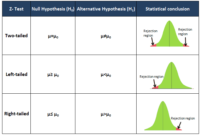
Null Hypothesis (H₀): Always states the population proportion equals a specific value.

\( H_0 : p = p_0 \)

Alternative Hypothesis (Hₐ): Depends on the claim:

One-Sided Test:

  • \( H_a : p > p_0 \) → right-tailed (testing if proportion is greater)
  • \( H_a : p < p_0 \) → left-tailed (testing if proportion is smaller)

Two-Sided Test:

  • \( H_a : p \neq p_0 \) → two-tailed (testing if proportion is different in either direction)

Step 2: Verify Conditions

  • Random: Data come from a random sample or randomized experiment.
  • Independence: Observations are independent. If sampling without replacement, check the 10% condition: \( n \leq 0.1N \).
  • Normal Approximation: The sample is large enough to use a Normal model.
    • Check: \( n p_0 \geq 10 \) and \( n(1 – p_0) \geq 10 \).

Step 3: Test Statistic

\( z = \dfrac{\hat{p} – p_0}{\sqrt{\dfrac{p_0 (1 – p_0)}{n}}} \)

  • \( \hat{p} = \dfrac{x}{n} \) = sample proportion
  • \( p_0 \) = hypothesized population proportion

Step 4: P-value and Decision

  • Find the P-value from the standard Normal distribution, depending on the alternative hypothesis.
  • Compare the P-value to the significance level \( \alpha \).
  • If P-value ≤ \( \alpha \), reject \( H_0 \). Otherwise, fail to reject \( H_0 \).

Example :

A company advertises that 80% of its customers are satisfied. In a random sample of 100 customers, 74 say they are satisfied. At the 5% significance level, do the data provide evidence that the satisfaction rate is less than advertised?

▶️ Answer / Explanation

Step 1: Hypotheses:

\( H_0 : p = 0.80 \)
\( H_a : p < 0.80 \) (left-tailed, one-sided).

Step 2: Conditions:

  • Random sample assumed.
  • 10% condition: \( 100 \leq 0.1N \) (reasonable for a large customer base).
  • Normal approximation: \( n p_0 = 100(0.8) = 80 \geq 10 \), \( n(1 – p_0) = 100(0.2) = 20 \geq 10 \).

Step 3: Test statistic:

\( \hat{p} = \dfrac{74}{100} = 0.74 \)

\( z = \dfrac{0.74 – 0.80}{\sqrt{\dfrac{0.8(0.2)}{100}}} = \dfrac{-0.06}{\sqrt{0.0016}} = \dfrac{-0.06}{0.04} = -1.5 \)

Step 4: P-value = \( P(Z < -1.5) \approx 0.067 \).

Conclusion: Since P-value (0.067) > 0.05, we fail to reject \( H_0 \). There is not enough evidence at the 5% level to conclude that customer satisfaction is less than 80%.

Example:

A manufacturer claims that 90% of its batteries last at least 6 hours. A consumer group suspects the proportion is less than this. State the hypotheses.

▶️ Answer / Explanation

Parameter: Let \( p = \) true proportion of batteries that last at least 6 hours.

Null Hypothesis: \( H_0 : p = 0.90 \)

Alternative Hypothesis: \( H_a : p < 0.90 \) (left-tailed, because the suspicion is “less than”).

Example:

A polling organization claims that exactly 50% of voters support a new law. An opposition group believes the support level is different. State the hypotheses.

▶️ Answer / Explanation

Parameter: Let \( p = \) true proportion of voters who support the new law.

Null Hypothesis: \( H_0 : p = 0.50 \)

Alternative Hypothesis: \( H_a : p \neq 0.50 \) (two-tailed, because the group suspects “different,” not specifically higher or lower).

Identifying an Appropriate Testing Method for a Population Proportion

Identifying an Appropriate Testing Method for a Population Proportion

When to Use: A 1-sample z-test for a population proportion is appropriate when you want to test a claim about the proportion of a categorical outcome in a population.

Key Features:

  • Parameter of Interest: The population proportion \( p \).
  • Data Type: Categorical (success/failure, yes/no, etc.).
  • Sample Size: A single random sample of size \( n \).
  • Null Hypothesis: Always of the form \( H_0 : p = p_0 \).
  • Alternative Hypothesis: One-sided (\( p > p_0 \) or \( p < p_0 \)) or two-sided (\( p \neq p_0 \)).

Conditions to Check:

  • Random: Sample comes from random sampling or a randomized experiment.
  • Independence: If sampling without replacement, check \( n \leq 0.1N \).
  • Normal Approximation: The sampling distribution of \( \hat{p} \) is approximately Normal if \( n p_0 \geq 10 \) and \( n(1 – p_0) \geq 10 \).

Test Statistic:

\( z = \dfrac{\hat{p} – p_0}{\sqrt{\dfrac{p_0 (1 – p_0)}{n}}} \)

Decision Rule:

  • Find the P-value from the z test statistic using the standard Normal distribution.
  • Compare to the significance level \( \alpha \).
  • If P-value ≤ \( \alpha \), reject \( H_0 \); otherwise, fail to reject \( H_0 \).

Example:

A candidate claims that 60% of voters support her. In a random sample of 150 voters, 78 say they support her. Is a 1-sample z-test for a population proportion appropriate here?

▶️ Answer / Explanation

Step 1: Parameter: Let \( p = \) true proportion of voters who support the candidate.

Step 2: Hypotheses: \( H_0 : p = 0.60 \), \( H_a : p \neq 0.60 \).

Step 3: Conditions: Random sample assumed. Independence: 150 ≤ 0.1N (population large). Normal approximation: \( n p_0 = 150(0.6) = 90 \geq 10 \), \( n(1-p_0) = 150(0.4) = 60 \geq 10 \).

Conclusion: All conditions are satisfied, so a 1-sample z-test for a population proportion is appropriate.

Verifying Conditions for Testing a Population Proportion

Verifying Conditions for Testing a Population Proportion

Before performing a one-sample z-test for a population proportion, we must ensure the assumptions for statistical inference are satisfied. There are two main checks: independence and approximate normality of the sampling distribution.

1. Independence:

  • Data should come from a random sample or a randomized experiment.
  • If sampling without replacement, check the 10% condition: \( n \leq 0.1N \), where \( N \) is the population size.

2. Normal Approximation (Shape of Sampling Distribution):

  • Assume the null hypothesis \( H_0: p = p_0 \) is true.
  • Check the success-failure condition:
    • Number of successes: \( n p_0 \geq 10 \)
    • Number of failures: \( n (1 – p_0) \geq 10 \)
  • If both are satisfied, the sample size is large enough to assume the sampling distribution of \( \hat{p} \) is approximately Normal.

Summary: Only if both independence and normal approximation conditions are met can we perform a one-sample z-test for a population proportion confidently.

Example:

A school claims that 70% of students participate in extracurricular activities. A random sample of 120 students is taken. Verify if a one-sample z-test for the population proportion is appropriate.

▶️ Answer / Explanation

Step 1: Independence

  • Data come from a random sample. 
  • 10% condition: 120 ≤ 0.1N (assuming total students N ≥ 1200). 

Step 2: Normal Approximation

  • Assume \( H_0: p = 0.70 \).
  • Number of successes: \( n p_0 = 120 * 0.70 = 84 \geq 10 \) 
  • Number of failures: \( n (1 – p_0) = 120 * 0.30 = 36 \geq 10 \) 

Conclusion: Both conditions satisfied. A one-sample z-test for a population proportion is appropriate.

Example 

A startup claims that 95% of users like their app. A random sample of 15 users is taken. Verify conditions for a one-sample z-test.

▶️ Answer / Explanation

Step 1: Independence

  • Random sample assumed. 
  • 10% condition: 15 ≤ 0.1N (likely satisfied). 

Step 2: Normal Approximation

  • Assume \( H_0: p = 0.95 \)
  • Number of successes: \( n p_0 = 15 * 0.95 = 14.25 < 10 \)? Actually, 14.25 ≥ 10 
  • Number of failures: \( n (1 – p_0) = 15 * 0.05 = 0.75 < 10 

Conclusion: Normal approximation condition not satisfied (few failures). A one-sample z-test is not appropriate. Use an exact test (like a binomial test) instead.

Scroll to Top