Home / AP Statistics 6.7 Potential Errors When Performing Tests Study Notes

AP Statistics 6.7 Potential Errors When Performing Tests Study Notes

AP Statistics Link Study Notes- New syllabus

AP Statistics Link Study Notes -As per latest AP Statistics Syllabus.

LEARNING OBJECTIVE

  • Probabilities of Type I and Type II errors influence inference.

Key Concepts:

  • Type I and Type II Errors in Hypothesis Testing
  • Calculating Probabilities of Type I and Type II Errors
  • Factors Affecting the Probability of Errors in Significance Testing
  • Interpreting Type I and Type II Errors

AP Statistics -Concise Summary Notes- All Topics

Type I and Type II Errors in Hypothesis Testing

Type I and Type II Errors in Hypothesis Testing

In hypothesis testing, two types of errors can occur when making a decision about the null hypothesis (\( H_0 \)) based on sample data:

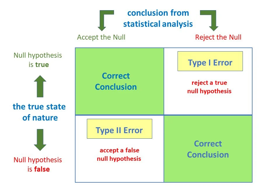
  • Type I Error: Rejecting \( H_0 \) when it is actually true.
  • Type II Error: Failing to reject \( H_0 \) when \( H_a \) is actually true.

Significance Level and Errors:

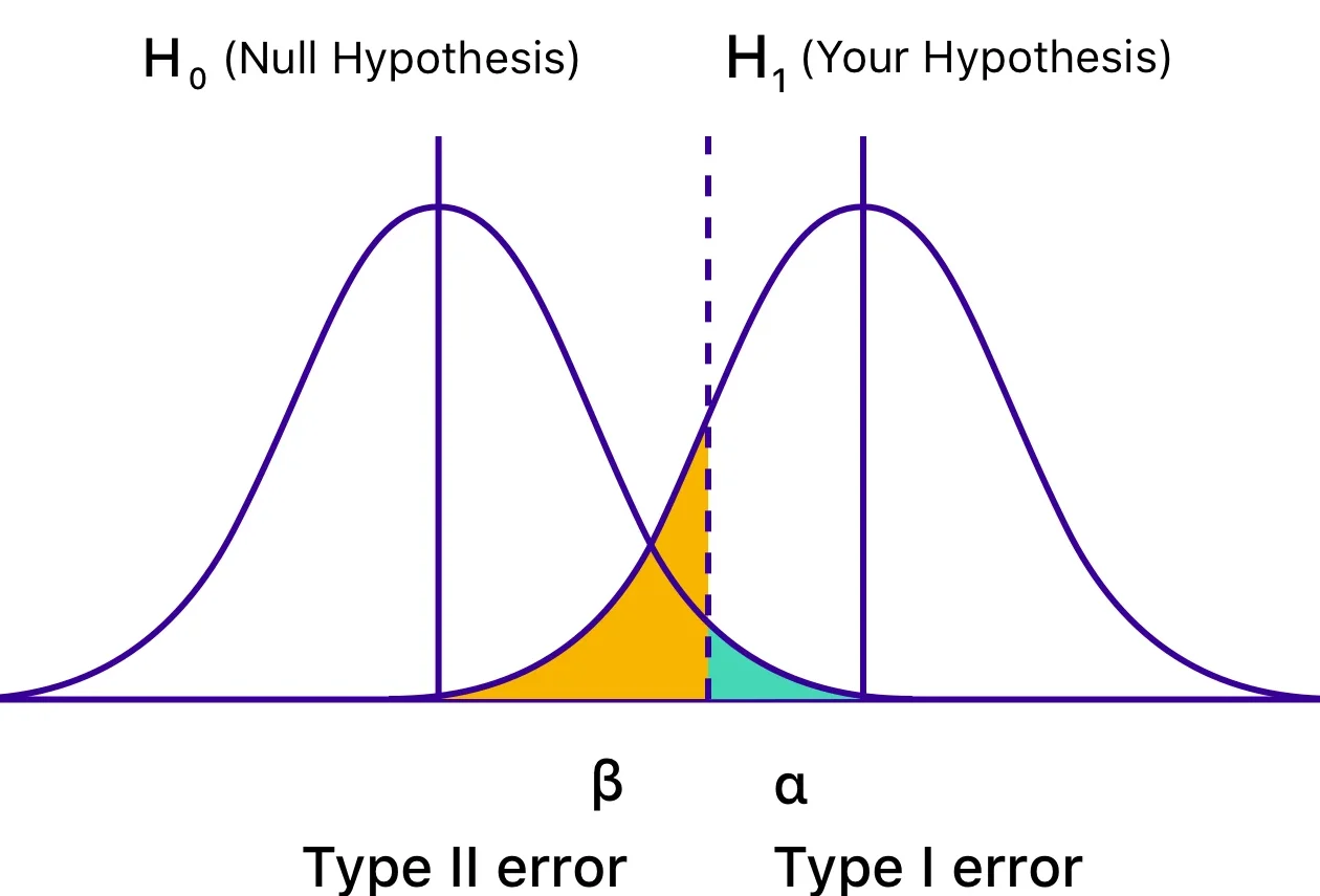
  • The probability of a Type I error is equal to the significance level \( \alpha \).
  • The probability of a Type II error is denoted by \( \beta \).
  • Smaller \( \alpha \) → less chance of Type I error, but may increase Type II error.

Table of Errors:

DecisionTrue State of NatureOutcome / Error
Reject \( H_0 \)\( H_0 \) is trueType I Error
Reject \( H_0 \)\( H_a \) is trueCorrect Decision
Fail to Reject \( H_0 \)\( H_0 \) is trueCorrect Decision
Fail to Reject \( H_0 \)\( H_a \) is trueType II Error

Notes:

  • Type I error is controlled by setting the significance level \( \alpha \).
  • Type II error (\( \beta \)) depends on the sample size, effect size, and \( \alpha \).
  • Reducing \( \alpha \) lowers the chance of Type I error but may increase Type II error unless the sample size is increased.
  • Always interpret errors in context of the population and research question.

Example :

A factory claims that at least 95% of its light bulbs last 1000 hours. A random sample of 50 bulbs is tested.

Scenario: The true proportion of bulbs lasting 1000 hours is actually 0.95.

Identify what a Type I and Type II error would represent in this situation.

▶️ Answer / Explanation

Type I Error: Rejecting the factory’s claim (H₀: p = 0.95) when it is actually true — concluding the bulbs do not meet the 95% standard when they actually do.

Type II Error: Failing to reject H₀ when the true proportion is actually less than 0.95 — concluding the bulbs meet the 95% standard when they do not.

Example :

A school claims that 80% of students pass a standardized test. A random sample of 60 students is tested.

Scenario: The true pass rate is actually 0.70.

 Identify what a Type I and Type II error would represent in this context.

▶️ Answer / Explanation

Type I Error: Rejecting the school’s claim (H₀: p = 0.80) when it is actually true — concluding that fewer than 80% of students pass when the true pass rate is 80%.

Type II Error: Failing to reject H₀ when the true pass rate is 70% — concluding that 80% of students pass when in reality fewer do.

Calculating Probabilities of Type I and Type II Errors

Calculating Probabilities of Type I and Type II Errors

Type I Error (\( \alpha \)):

The probability of rejecting the null hypothesis \( H_0 \) when it is true.

  • Significance level (\( \alpha \)) is the maximum allowable probability of making a Type I error.
  • For a z-test (one-sample proportion):

Right-tailed test: \( \alpha = P(Z > z_\alpha) \)
Left-tailed test: \( \alpha = P(Z < z_\alpha) \)
Two-tailed test: \( \alpha = P(Z < -z_{\alpha/2}) + P(Z > z_{\alpha/2}) \)

 Type II Error (\( \beta \)):

 The probability of failing to reject \( H_0 \) when the alternative \( H_a \) is true.

  • \( \beta \) depends on:
    • The true population proportion under \( H_a \)
    • Sample size \( n \)
    • Significance level \( \alpha \)
  • Formula for one-sample z-test (proportion):

\( \beta = P(\text{Fail to reject } H_0 \mid p = p_a) = P(z \text{ within non-rejection region under } p_a) \)

Stepwise Approach to Compute \( \beta \):

  1. Determine the rejection region based on \( \alpha \) and \( H_0 \).
  2. Find the z-scores corresponding to the non-rejection region assuming \( p = p_a \) (true proportion under \( H_a \)).
  3. Compute the probability that the sample statistic falls within this non-rejection region; this is \( \beta \).

Example:

A factory claims that 95% of light bulbs last over 1000 hours. A sample of 50 bulbs is tested. Use a significance level of 0.05. Suppose the true proportion is 90%. Calculate \( \alpha \) and \( \beta \) for a left-tailed test.

▶️ Answer / Explanation

Step 1: Type I error (\( \alpha \))

Left-tailed test → rejection region: \( z < -z_{0.05} = -1.645 \)

\( \alpha = P(Z < -1.645 \mid p_0 = 0.95) = 0.05 \)

Step 2: Type II error (\( \beta \))

    • True proportion under \( H_a \): \( p_a = 0.90 \)
    • Compute mean and standard error under \( p_a \):

SE = \( \sqrt{p_a(1-p_a)/n} = \sqrt{0.90*0.10/50} \approx 0.0424 \)

    • Find z-score for the non-rejection boundary under \( p_a \):

z = \( \dfrac{p_\text{crit} – p_a}{SE} \), where \( p_\text{crit} = p_0 + z_\alpha * \sqrt{p_0(1-p_0)/n} \)

p_crit = 0.95 + (-1.645)*√(0.95*0.05/50) ≈ 0.936

z = (0.936 – 0.90)/0.0424 ≈ 0.849

β = P(Z < 0.849) ≈ 0.802

Step 3: Interpretation

α = 0.05 → 5% chance of rejecting the factory’s claim when true.

β ≈ 0.802 → 80.2% chance of failing to reject the claim when the true proportion is actually 90%.

Factors Affecting the Probability of Errors in Significance Testing

Factors Affecting the Probability of Errors in Significance Testing

In hypothesis testing, the probabilities of Type I and Type II errors depend on several key factors:

1. Significance Level (\( \alpha \))

  • Type I error (\( \alpha \)) is directly controlled by the chosen significance level.
  • Lowering \( \alpha \) reduces the chance of a Type I error but may increase the probability of a Type II error (\( \beta \)).

2. Sample Size (\( n \))

  • Larger sample sizes reduce the standard error, making the sampling distribution narrower.
  • This reduces \( \beta \) (Type II error), increasing the test’s power, without affecting \( \alpha \).

3. Effect Size

  • The difference between the true population parameter and the value stated in \( H_0 \).
  • Larger effect sizes make it easier to detect a difference, decreasing \( \beta \) (increasing power).

4. Variability in the Population

  • Greater population variability increases the standard error, making it harder to detect a true effect.
  • This increases \( \beta \) and decreases the power of the test.

5. Direction of the Test

  • One-tailed vs two-tailed tests affect the rejection region.
  • A one-tailed test concentrates the α in one direction, reducing the critical value and increasing power for an effect in that direction.

Example:

A researcher wants to test if a new teaching method improves test scores. Discuss how each of the following would affect the probabilities of Type I and Type II errors:

  • Increasing the sample size
  • Lowering the significance level from 0.05 to 0.01
  • The true improvement in scores is very small
▶️ Answer / Explanation
  • Increasing sample size: Reduces standard error → decreases β → more power → Type I error unaffected
  • Lowering α: Reduces Type I error → makes rejection region smaller → increases β → less power
  • Small true effect: Harder to detect → β increases → less power → Type I error unaffected

Interpreting Type I and Type II Errors

Interpreting Type I and Type II Errors

Type I and Type II errors are mistakes that can occur when making decisions based on sample data:

  • Type I Error (α): Rejecting the null hypothesis \( H_0 \) when it is actually true.
  • Type II Error (β): Failing to reject \( H_0 \) when the alternative hypothesis \( H_a \) is actually true.

Contextual Interpretation:

  • Whether a Type I or Type II error is more serious depends on the situation and consequences of making each error.
  • Examples:
    • Medical testing: Type I error = diagnosing a healthy patient as sick; Type II error = failing to diagnose a sick patient.
    • Quality control: Type I error = rejecting a batch of good products; Type II error = accepting a batch of defective products.

Role of Significance Level (α):

  • The significance level is the probability of making a Type I error.
  • When Type I errors are more consequential, researchers may choose a smaller α (e.g., 0.01 instead of 0.05).
  • Choosing α involves balancing the risk of Type I and Type II errors based on the context.

Summary:

  • Type I error: false positive → reject true null hypothesis.
  • Type II error: false negative → fail to reject false null hypothesis.
  • Consequences of errors guide the choice of significance level and study design.

Example:

A hospital tests a new drug to reduce blood pressure. The null hypothesis is that the drug has no effect. Interpret Type I and Type II errors in this context and explain which might be more serious.

▶️ Answer / Explanation
  • Type I Error: Concluding that the drug works when it actually does not → might lead to giving patients an ineffective treatment.
  • Type II Error: Concluding that the drug does not work when it actually does → might prevent patients from receiving a beneficial treatment.
  • More consequential: Depending on context, a Type II error may be worse if patients miss an effective treatment, or a Type I error may be worse if side effects of an ineffective drug are serious.
  • The choice of α should reflect which error is more critical.
Scroll to Top