Interpret a Confidence Interval for a Difference of Proportions
A confidence interval for the difference in population proportions \( p_1 – p_2 \) provides a range of plausible values for the true difference between two populations. It reflects how confident we are that this interval captures the actual difference in proportions.
- The interval is based on the sample data (\( \hat{p}_1, \hat{p}_2 \)) and accounts for sampling variability.
- The form of the interval is:
\( (\hat{p}_1 – \hat{p}_2) \pm z^* \sqrt{\dfrac{\hat{p}_1 (1 – \hat{p}_1)}{n_1} + \dfrac{\hat{p}_2 (1 – \hat{p}_2)}{n_2}} \)
Interpretation:
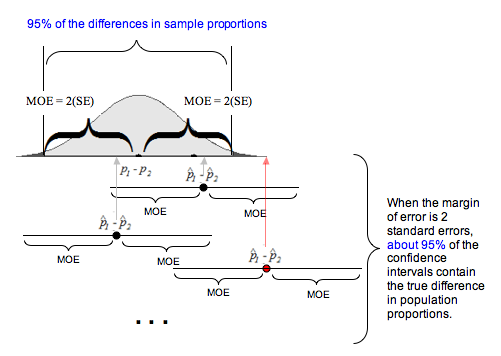
- We are C% confident that the true difference in population proportions \( p_1 – p_2 \) lies within the calculated interval.
- In repeated random sampling with the same sample sizes, about C% of such intervals would capture the true difference.
- The interpretation must always refer to:
- the populations being compared,
- the parameters of interest (\( p_1 – p_2 \)), and
- the context of the situation.
Example:
A survey found that 60% of urban residents and 52% of rural residents support recycling incentives. A 95% confidence interval for \( p_1 – p_2 \) (urban − rural) is calculated as (0.01, 0.15).
Interpret the confidence interval.
▶️ Answer / Explanation
- We are 95% confident that the true difference in proportions of urban and rural residents who support recycling lies between 0.01 and 0.15.
- This means that the proportion of urban supporters is likely between 1% and 15% higher than that of rural supporters.
- In repeated random sampling, about 95% of such intervals would capture the true difference in support rates.