AP Statistics 7.2 Constructing a Confidence Interval for a Population Mean Study Notes
AP Statistics 7.2 Constructing a Confidence Interval for a Population Mean Study Notes- New syllabus
AP Statistics 7.2 Constructing a Confidence Interval for a Population Mean Study Notes -As per latest AP Statistics Syllabus.
LEARNING OBJECTIVE
- The t-distribution may be used to model variation.
Key Concepts:
- Describing t-Distributions
- Identifying an Appropriate Confidence Interval Procedure for a Population Mean
- Verifying Conditions for Confidence Intervals for a Population Mean
- Critical t-Value and Standard Error for a Sample Mean
- Confidence Interval for a Population Mean
Describing t-Distributions
The t-distribution is a family of probability distributions that arise when estimating a population mean using a sample mean, particularly when the population standard deviation (\(\sigma\)) is unknown.
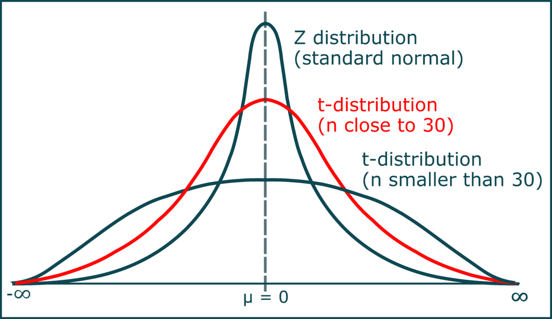
- Shape: Symmetric and bell-shaped, like the standard normal distribution (\(N(0,1)\)).
- Spread: Wider (heavier tails) than the standard normal distribution, reflecting extra variability from estimating \(\sigma\).
- Degrees of freedom (df): The exact shape depends on \(df = n – 1\) for a sample of size \(n\). Smaller \(df\) = thicker tails.
- Convergence: As \(df \to \infty\), the t-distribution approaches the standard normal distribution.
- Use: Commonly applied in confidence intervals and hypothesis tests for means when \(\sigma\) is unknown.
Example
A researcher wants to estimate the average height of college students. They collect a random sample of \(n = 12\) students, compute a sample mean height \(\bar{x} = 170 \, \text{cm}\), and a sample standard deviation \(s = 8 \, \text{cm}\).
▶️ Answer / Explanation
Because the population standard deviation \(\sigma\) is unknown, the researcher must use a t-distribution with \(df = n – 1 = 11\) when constructing confidence intervals or performing hypothesis tests.
The test statistic for a hypothesis test about the mean would be calculated as:
\( t = \dfrac{\bar{x} – \mu_0}{s / \sqrt{n}} \)
This statistic follows a t-distribution with \(df = 11\). The heavier tails of the t-distribution reflect the uncertainty due to estimating \(\sigma\) from the sample.
The t-Distribution for a Sample Mean
When we have a single quantitative variable \(X\) that is normally distributed but the population standard deviation \(\sigma\) is unknown, we use the sample mean \(\bar{x}\) and the sample standard deviation \(s\) to form a standardized statistic.
Test statistic:
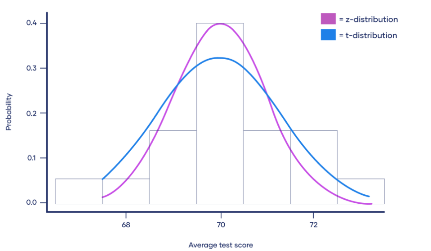
\( t = \dfrac{\bar{x} – \mu}{s / \sqrt{n}} \)
- \(\bar{x}\) = sample mean
- \(\mu\) = hypothesized population mean
- \(s\) = sample standard deviation
- \(n\) = sample size
Distribution:
- This statistic follows a t-distribution with \(df = n – 1\) degrees of freedom.
- The t-distribution is symmetric and bell-shaped like the normal distribution, but has heavier tails.
- As \(n\) increases, the t-distribution approaches the standard normal distribution.
Example
A company claims the average weight of its snack packs is 50 grams. A sample of \(n = 16\) packs has mean \(\bar{x} = 48.5\) grams and standard deviation \(s = 2.4\) grams. Test whether the mean weight differs from 50 grams.
▶️ Answer / Explanation
We compute:
\( t = \dfrac{48.5 – 50}{2.4 / \sqrt{16}} = \dfrac{-1.5}{0.6} = -2.5 \)
Degrees of freedom: \(df = 16 – 1 = 15\).
Using a t-table or calculator, the p-value (two-sided) is approximately 0.025.
Conclusion: At significance level \(\alpha = 0.05\), we reject \(H_0\). The data provide evidence that the true mean snack pack weight is different from 50 g.
Identifying an Appropriate Confidence Interval Procedure for a Population Mean
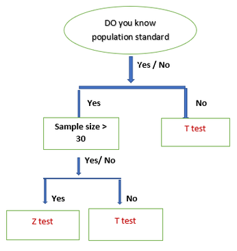
When constructing a confidence interval for a population mean, the correct procedure depends on whether the population standard deviation \(\sigma\) is known:
- If \(\sigma\) is known: Use a z-interval for the mean.
- If \(\sigma\) is unknown: Use a t-interval for the mean with \(df = n – 1\).
Matched pairs scenario:
- For data in matched pairs (e.g., before-and-after studies or paired subjects), compute the differences for each pair.
- Treat these differences as a single sample of size \(n\).
- Construct a one-sample t-interval for the mean difference.
General formula:
\( \bar{x} \pm t^* \dfrac{s}{\sqrt{n}} \)
- \(\bar{x}\) = sample mean (or mean of differences in matched pairs)
- \(s\) = sample standard deviation
- \(n\) = sample size (or number of pairs)
- \(t^*\) = critical value from t-distribution with \(df = n-1\)
Example
A researcher measures the blood pressure of 10 patients before and after taking a new medication. The differences (after – before) have a mean \(\bar{d} = -5 \, \text{mmHg}\), standard deviation \(s_d = 6 \, \text{mmHg}\), and \(n = 10\).
We want a 95% confidence interval for the mean difference in blood pressure.
▶️ Answer / Explanation
Since this is a matched pairs design, we use a one-sample t-interval for the differences:
CI = \(\bar{d} \pm t^* \dfrac{s_d}{\sqrt{n}}\)
With \(df = 9\), \(t^* \approx 2.262\) for 95% confidence.
CI = \(-5 \pm 2.262 \dfrac{6}{\sqrt{10}}\)
CI = \(-5 \pm 4.29 \implies (-9.29, -0.71)\)
Interpretation: We are 95% confident that the mean decrease in blood pressure due to the medication is between 0.71 mmHg and 9.29 mmHg.
Verifying Conditions for Confidence Intervals for a Population Mean
Before constructing a confidence interval for a population mean, we must ensure the following conditions are met:
Random:
The data come from a random sample or a randomized experiment.
Independence:
Observations must be independent. If sampling without replacement, check the 10% condition: \( n \leq 0.1N \), where \(N\) is the population size.
Normality / Sample Size:
- For a one-sample CI, the variable should be approximately normally distributed in the population, or the sample size should be large enough (\(n \geq 30\)) for the Central Limit Theorem to apply.
- For matched pairs, calculate the differences first. The distribution of differences should be approximately normal, or the number of pairs should be large enough (\(n \geq 30\)).
Example
A nutritionist measures the weight of 12 participants before and after a 6-week diet program. The differences (after – before) are approximately symmetric, and the sample is randomly selected.
▶️ Answer / Explanation
Check conditions for a one-sample CI for the mean difference:
- Random: Data come from a random sample — satisfied.
- Independence: Each participant is independent; 12 is less than 10% of the population — satisfied.
- Normality: Differences are approximately symmetric and sample size is small (\(n = 12\)), so normality assumption is reasonable.
All conditions are met, so a t-interval can be used to estimate the mean weight change.
Critical t-Value and Standard Error for a Sample Mean
When constructing a confidence interval for a population mean or performing a t-test, two key components are used: the critical t-value and the standard error of the mean.
Critical t-value (\(t^*\)): The value from the t-distribution with \(df = n – 1\) that corresponds to the desired confidence level.
- Can be found using a t-table or computer-generated output.
- Accounts for the extra variability due to estimating the population standard deviation using the sample standard deviation.
Standard Error (SE) of the Sample Mean: Measures the expected variability of the sample mean around the population mean.
\( SE = \dfrac{s}{\sqrt{n}} \)
- \(s\) = sample standard deviation
- \(n\) = sample size
Using these two quantities, the margin of error for a confidence interval can be calculated:
\( ME = t^* \cdot SE = t^* \dfrac{s}{\sqrt{n}} \)
Example
A random sample of \(n = 20\) measurements has a sample mean \(\bar{x} = 55\) and standard deviation \(s = 8\). Find the 95% confidence interval using the critical t-value.
▶️ Answer / Explanation
Step 1: Degrees of freedom: \(df = n – 1 = 19\).
Step 2: For 95% confidence, \(t^* \approx 2.093\).
Step 3: Standard error: \( SE = \dfrac{s}{\sqrt{n}} = \dfrac{8}{\sqrt{20}} \approx 1.789 \).
Step 4: Margin of error: \( ME = t^* \cdot SE = 2.093 \cdot 1.789 \approx 3.74 \).
Step 5: Confidence interval: \( \bar{x} \pm ME = 55 \pm 3.74 = (51.26, 58.74) \).
Confidence Interval for a Population Mean
The point estimate for a population mean is the sample mean \(\bar{x}\). When the population standard deviation \(\sigma\) is unknown, we use the sample standard deviation \(s\) and the t-distribution to calculate a confidence interval.
Formula for a one-sample t-interval:
\( \bar{x} \pm t^* \dfrac{s}{\sqrt{n}} \)
- \(\bar{x}\) = sample mean (point estimate of \(\mu\))
- \(s\) = sample standard deviation
- \(n\) = sample size
- \(t^*\) = critical value from t-distribution with \(df = n – 1\)
For matched pairs: Calculate the differences \(d = X_{\text{after}} – X_{\text{before}}\) first, then compute \(\bar{d}\) and \(s_d\). The confidence interval for the mean difference is:
\( \bar{d} \pm t^* \dfrac{s_d}{\sqrt{n}} \)
- \(\bar{d}\) = mean of the differences
- \(s_d\) = standard deviation of the differences
- \(n\) = number of paired observations
- \(t^*\) = critical value from t-distribution with \(df = n – 1\)
Example
A nutritionist measures the weight of 10 participants before and after a 6-week diet program. The differences (after – before) have a mean \(\bar{d} = -2.4\) kg and standard deviation \(s_d = 1.2\) kg. Find the 95% confidence interval for the mean weight change.
▶️ Answer / Explanation
Step 1: Degrees of freedom: \(df = n – 1 = 10 – 1 = 9\).
Step 2: For 95% confidence, \(t^* \approx 2.262\).
Step 3: Standard error: \( SE = \dfrac{s_d}{\sqrt{n}} = \dfrac{1.2}{\sqrt{10}} \approx 0.379 \).
Step 4: Margin of error: \( ME = t^* \cdot SE = 2.262 \cdot 0.379 \approx 0.857 \).
Step 5: Confidence interval: \( \bar{d} \pm ME = -2.4 \pm 0.857 = (-3.257, -1.543) \) kg.
Interpretation: We are 95% confident that the diet program reduced the average weight by between 1.543 kg and 3.257 kg.