Home / AP Statistics 7.3 Justifying a Claim About a Population Mean Based on a Confidence Interval Study Notes

AP Statistics 7.3 Justifying a Claim About a Population Mean Based on a Confidence Interval Study Notes

AP Statistics 7.3 Justifying a Claim About a Population Mean Based on a Confidence Interval Study Notes- New syllabus

AP Statistics 7.3 Justifying a Claim About a Population Mean Based on a Confidence Interval Study Notes -As per latest AP Statistics Syllabus.

LEARNING OBJECTIVE

  • An interval of values should be used to estimate parameters, in order to account for uncertainty.

Key Concepts:

  • Understanding Confidence Intervals
  • Justifying a Claim Based on a Confidence Interval for a Population Mean
  • Relationships Between Sample Size, Confidence Interval Width, Confidence Level, and Margin of Error (Population Mean)

AP Statistics -Concise Summary Notes- All Topics

Understanding Confidence Intervals

Understanding Confidence Intervals

A confidence interval (CI) gives a range of values that is likely to contain a population parameter, such as a mean.

  • Imagine taking a random sample from a population and calculating its mean. Because the sample is just one of many possible samples, the mean could be slightly higher or lower than the true population mean.
  • The confidence interval accounts for this uncertainty by giving a range around the sample mean.

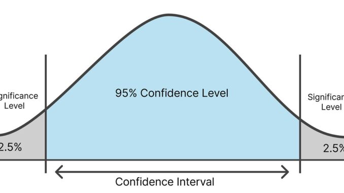
What “C% confident” means

  • “We are C% confident” does not mean there is a C% chance the true mean is in this specific interval.
  • It means that if we repeated the sampling process many times, about C% of the intervals would contain the true population mean.
  • Each individual interval either does or does not contain the true mean; we just don’t know which one.

Interpreting a CI for Matched Pairs

Matched pairs arise when measuring the same subjects under two conditions (e.g., before and after).

  1. Compute the difference for each pair.
  2. Treat these differences as a new sample.
  3. Calculate the CI for the mean difference.
  • If the CI for the mean difference does not include 0, it suggests a real change between conditions.
  • We can say: “We are C% confident that the true average difference in the population lies in this interval.”

Summary

  • CI = range of plausible values for a population parameter.
  • “C% confident” = method would capture the true mean in C% of repeated samples.
  • Matched pairs = focus on mean differences.

Example

A teacher wants to estimate the average improvement in test scores for 12 students after a special tutoring program. The “after – before” differences in scores have a mean \(\bar{d} = 8.5\) points and standard deviation \(s_d = 3.2\) points. Find the 95% confidence interval for the mean improvement.

▶️ Answer / Explanation

Step 1: Degrees of freedom: \(df = n – 1 = 12 – 1 = 11\).

Step 2: For 95% confidence, \(t^* \approx 2.201\).

Step 3: Standard error: \( SE = \dfrac{s_d}{\sqrt{n}} = \dfrac{3.2}{\sqrt{12}} \approx 0.924 \).

Step 4: Margin of error: \( ME = t^* \cdot SE = 2.201 \cdot 0.924 \approx 2.03 \).

Step 5: Confidence interval: \( \bar{d} \pm ME = 8.5 \pm 2.03 = (6.47, 10.53) \) points.

Interpretation: We are 95% confident that the tutoring program increased the average test score by between 6.47 and 10.53 points.

Justifying a Claim Based on a Confidence Interval for a Population Mean

Justifying a Claim Based on a Confidence Interval for a Population Mean

A confidence interval provides a range of plausible values for a population parameter. It can be used to justify or evaluate a claim about the population mean (\(\mu\)) or the mean difference in matched pairs (\(\mu_d\)).

  • If a hypothesized value (e.g., \(\mu_0\)) lies inside the confidence interval, there is insufficient evidence to reject the claim.
  • If a hypothesized value lies outside the confidence interval, there is evidence to suggest the claim may not be true.
  • Matched pairs: first calculate differences \(d = X_{\text{after}} – X_{\text{before}}\), then construct a confidence interval for \(\mu_d\). The same interpretation applies to \(\mu_d\).
  • Always state conclusions in context, referring to the population and the sample.

Example

A study claims a training program improves test scores by 5 points on average. A random sample of 12 participants shows differences (after – before) with a mean \(\bar{d} = 6\) and standard deviation \(s_d = 2\). Construct a 95% confidence interval for the mean improvement and justify whether the program meets the claimed improvement.

▶️ Answer / Explanation

Step 1: Degrees of freedom: \(df = n – 1 = 12 – 1 = 11\).

Step 2: For 95% confidence, \(t^* \approx 2.201\).

Step 3: Standard error: \( SE = \dfrac{s_d}{\sqrt{n}} = \dfrac{2}{\sqrt{12}} \approx 0.577 \).

Step 4: Margin of error: \( ME = t^* \cdot SE = 2.201 \cdot 0.577 \approx 1.27 \).

Step 5: Confidence interval: \( \bar{d} \pm ME = 6 \pm 1.27 = (4.73, 7.27) \).

Conclusion: The 95% confidence interval for the mean improvement is 4.73 to 7.27 points. Since the claimed improvement of 5 points lies within this interval, the data provide support for the program meeting its claim. The conclusion is stated in context, referencing the participants in the study.

Relationships Between Sample Size, Confidence Interval Width, Confidence Level, and Margin of Error

Relationships Between Sample Size, Confidence Interval Width, Confidence Level, and Margin of Error (Population Mean)

The width of a confidence interval (CI) for a population mean depends on several factors, which also affect the margin of error (ME):

Sample Size (\(n\)):

  • The standard error of the mean: \( SE = \dfrac{s}{\sqrt{n}} \).
  • As \(n\) increases, \(SE\) decreases, which decreases \(ME = t^* \cdot SE\) and narrows the confidence interval.
  • Conclusion: Larger samples provide more precise estimates of the population mean.

Confidence Level (C%):

  • The critical t-value \(t^*\) increases with higher confidence levels.
  • For a given sample size, a higher confidence level → larger \(t^*\) → larger margin of error → wider confidence interval.
  • Conclusion: There is a trade-off between confidence level and interval width; more confidence means less precision.

Width of the Interval:

  • Width = \( 2 \cdot ME = 2 \cdot t^* \cdot \dfrac{s}{\sqrt{n}} \).
  • For a single mean, the width of the interval is directly proportional to the critical t-value (\(t^*\)) and standard deviation (\(s\)), and inversely proportional to \(\sqrt{n}\).
  • Therefore, increasing sample size narrows the interval, while increasing confidence level widens it.

Example

A researcher wants a 90% confidence interval for the mean height of students. The sample has \(n = 36\), \(\bar{x} = 170\) cm, and \(s = 6\) cm. If the researcher increases the confidence level to 99%, what happens to the width of the interval?

▶️ Answer / Explanation

Step 1: Standard error: \( SE = \dfrac{s}{\sqrt{n}} = \dfrac{6}{\sqrt{36}} = 1 \).

Step 2: Critical t-value for 90% CI with \(df = 35\): \( t^* \approx 1.690 \).

Step 3: Margin of error: \( ME_{90} = 1.690 \cdot 1 = 1.69 \).

Step 4: For 99% CI, \( t^* \approx 2.724 \), so \( ME_{99} = 2.724 \cdot 1 = 2.724 \).

Step 5: Width of intervals: – 90% CI: \( 2 \cdot ME = 3.38 \) cm – 99% CI: \( 2 \cdot ME = 5.448 \) cm

Conclusion: Increasing the confidence level widens the confidence interval, reflecting greater uncertainty required for higher confidence.

Scroll to Top