Home / AP Statistics 7.4 Setting Up a Test for a Population Mean Study Notes

AP Statistics 7.4 Setting Up a Test for a Population Mean Study Notes

AP Statistics 7.4 Setting Up a Test for a Population Mean Study Notes- New syllabus

AP Statistics 7.4 Setting Up a Test for a Population Mean Study Notes -As per latest AP Statistics Syllabus.

LEARNING OBJECTIVE

  • The t-distribution may be used to model variation.

Key Concepts:

  • Testing Methods for a Population Mean (Unknown \(\sigma\)) and Matched Pairs
  • Null and Alternative Hypotheses for a Population Mean (Unknown \(\sigma\)) and Matched Pairs
  • Verifying Conditions for a t-Test for a Population Mean (Unknown \(\sigma\)) and Matched Pairs

AP Statistics -Concise Summary Notes- All Topics

Testing Methods for a Population Mean (Unknown \(\sigma\)) and Matched Pairs

Testing Methods for a Population Mean (Unknown \(\sigma\)) and Matched Pairs

When the population standard deviation \(\sigma\) is unknown, we cannot use the z-test. Instead, we use a one-sample t-test based on the sample standard deviation \(s\). This applies to:

  • Single sample mean (\(\mu\)): Use a one-sample t-test.
  • Matched pairs / paired differences (\(\mu_d\)): Compute the differences \(d = X_{\text{after}} – X_{\text{before}}\) and perform a one-sample t-test on the differences.

Test statistic formula (single sample mean):

\( t = \dfrac{\bar{x} – \mu_0}{s / \sqrt{n}} \)

Test statistic formula (matched pairs / mean difference):

\( t = \dfrac{\bar{d} – \mu_{d,0}}{s_d / \sqrt{n}} \)

  • \(\bar{x}\) = sample mean, \(\bar{d}\) = mean of paired differences
  • \(\mu_0\) = hypothesized population mean, \(\mu_{d,0}\) = hypothesized mean difference
  • \(s\) = sample standard deviation, \(s_d\) = standard deviation of differences
  • \(n\) = sample size (or number of pairs)

Null distribution:

  • Under \(H_0\) and all conditions satisfied, the t-test statistic follows a t-distribution with \(df = n – 1\).
  • This distribution is used to calculate p-values and make decisions about the null hypothesis.

Example

A researcher claims a meditation program reduces stress scores by 5 points on average. A sample of 15 participants has mean reduction \(\bar{d} = 6.2\) with standard deviation \(s_d = 2.1\). Test at \(\alpha = 0.05\) whether the program reduces stress by more than 5 points.

▶️ Answer / Explanation

Step 1: Null and alternative hypotheses:

\( H_0: \mu_d = 5 \), \( H_a: \mu_d > 5 \) (one-sided test)

Step 2: Test statistic:

\( t = \dfrac{\bar{d} – \mu_{d,0}}{s_d / \sqrt{n}} = \dfrac{6.2 – 5}{2.1 / \sqrt{15}} = \dfrac{1.2}{0.542} \approx 2.21 \)

Step 3: Degrees of freedom: \( df = 15 – 1 = 14 \)

Step 4: Find p-value (t-distribution, one-sided): \( p \approx 0.023 \)

Step 5: Decision: \( p < 0.05 \) → reject \( H_0 \).

Conclusion: The data provide evidence that the meditation program reduces stress by more than 5 points on average.

Null and Alternative Hypotheses for a Population Mean (Unknown \(\sigma\)) and Matched Pairs

Null and Alternative Hypotheses for a Population Mean (Unknown \(\sigma\)) and Matched Pairs

When performing a t-test for a population mean (\(\mu\)) or the mean difference in matched pairs (\(\mu_d\)):

Single sample mean (\(\mu\)):

  • Null hypothesis: \(H_0: \mu = \mu_0\), where \(\mu_0\) is the hypothesized population mean.
  • Alternative hypothesis: Depends on the research question:
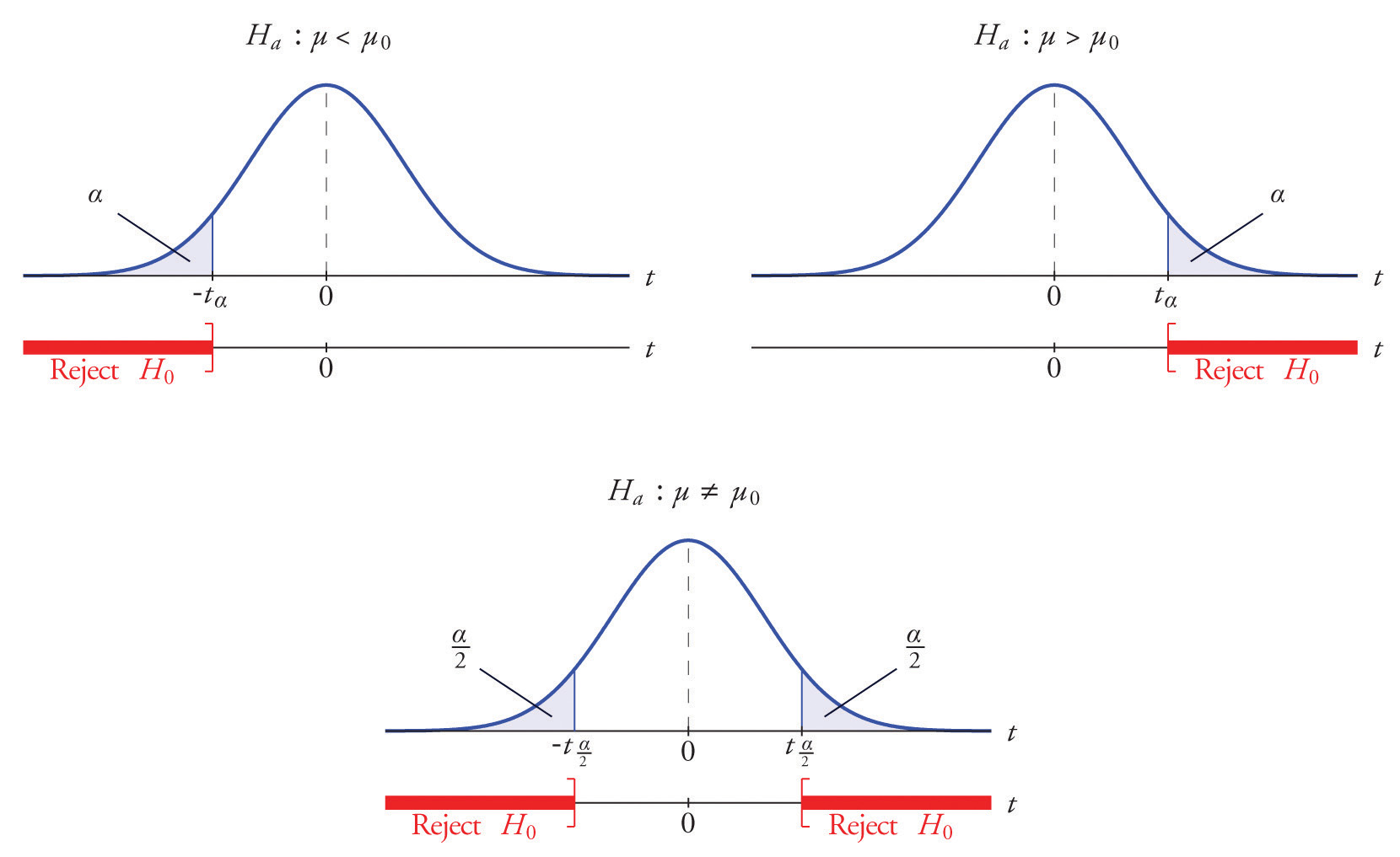
    • Two-sided: \(H_a: \mu \ne \mu_0\)
    • One-sided (greater): \(H_a: \mu > \mu_0\)
    • One-sided (less): \(H_a: \mu < \mu_0\)

Matched pairs / mean difference (\(\mu_d\)):

  • Compute differences: \(d = X_{\text{after}} – X_{\text{before}}\)
  • Null hypothesis: \(H_0: \mu_d = 0\) (or another claimed value)
  • Alternative hypothesis:
    • Two-sided: \(H_a: \mu_d \ne 0\)
    • One-sided (increase): \(H_a: \mu_d > 0\)
    • One-sided (decrease): \(H_a: \mu_d < 0\)

Example

A diet program claims to reduce average weight by 4 kg. A sample of 10 participants is measured before and after the program. Let \(d = \text{weight before} – \text{weight after}\). Identify the null and alternative hypotheses for testing the claim.

▶️ Answer / Explanation

Step 1: Define population parameter: \(\mu_d\) = true mean weight loss.

Step 2: Null hypothesis (claim to test): \(H_0: \mu_d = 4\)

Step 3: Alternative hypothesis (research question): If testing whether the program reduces more than claimed: \(H_a: \mu_d > 4\) If testing any difference: \(H_a: \mu_d \ne 4\) If testing if the reduction is less than claimed: \(H_a: \mu_d < 4\)

Step 4: State conclusion in context after performing the t-test.

Verifying Conditions for a t-Test for a Population Mean (Unknown \(\sigma\)) and Matched Pairs

Verifying Conditions for a t-Test for a Population Mean (Unknown \(\sigma\)) and Matched Pairs

Before performing a t-test for a single mean or for matched pairs, the following conditions must be checked to ensure valid statistical inference:

Randomness / Independence:

  • Data should come from a random sample or a randomized experiment.
  • If sampling without replacement, check the 10% condition: \( n \le 0.1N \), where \(N\) is the population size.
  • For matched pairs, each pair should be independent of other pairs.

Normality / Shape:

  • The sampling distribution of the mean or mean difference should be approximately normal.
  • Check the distribution of the data (or differences for paired data):
    • For small sample sizes (\(n < 30\)), the population or differences should be approximately normally distributed.
    • For larger sample sizes (\(n \ge 30\)), the Central Limit Theorem ensures approximate normality even if the population is not perfectly normal.

Example

A researcher wants to test whether a relaxation program reduces stress scores. A sample of 12 participants is measured before and after the program. What conditions must be verified before performing a t-test on the paired differences?

▶️ Answer / Explanation

Step 1: Randomness / Independence:

– Ensure the 12 participants were randomly selected or randomly assigned.

– Each participant’s response is independent of others.

Step 2: 10% condition:

– If participants were sampled without replacement, check that 12 ≤ 0.1 × population size. Likely satisfied if population is large.

Step 3: Normality / Shape:

– Sample size is small (\(n = 12 < 30\)), so we need to check the distribution of differences for approximate normality (no strong skew or outliers).

Conclusion: If all conditions are reasonably met, a one-sample t-test on the paired differences can be performed.

Scroll to Top