AP Statistics 7.6 Confidence Intervals for the Difference of Two Means Study Notes
AP Statistics 7.6 Confidence Intervals for the Difference of Two Means Study Notes- New syllabus
AP Statistics 7.6 Confidence Intervals for the Difference of Two Means Study Notes -As per latest AP Statistics Syllabus.
LEARNING OBJECTIVE
- An interval of values should be used to estimate parameters, in order to account for uncertainty
Key Concepts:
- Confidence Interval Procedure for a Difference of Two Population Means (\(\mu_1 – \mu_2\))
- Verifying Conditions for Confidence Intervals for a Difference of Two Population Means (\(\mu_1 – \mu_2\))
- Determining the Margin of Error for a Difference of Two Population Means (\(\mu_1 – \mu_2\))
- Confidence Interval Procedure for a Difference of Two Population Means (Unknown \(\sigma\))
Confidence Interval Procedure for a Difference of Two Population Means (\(\mu_1 - \mu_2\))
Confidence Interval Procedure for a Difference of Two Population Means (\(\mu_1 – \mu_2\))
Consider two independent populations:![]()
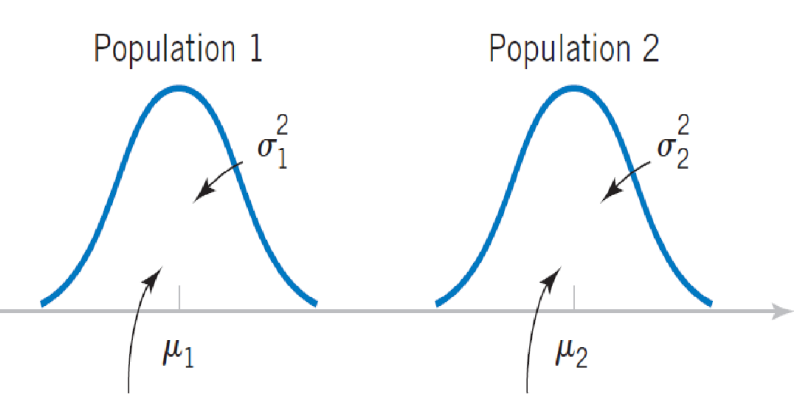
- Population 1: simple random sample of size \(n_1\), mean \(\bar{x}_1\), standard deviation \(s_1\)
- Population 2: simple random sample of size \(n_2\), mean \(\bar{x}_2\), standard deviation \(s_2\)
Conditions for using a two-sample t-interval:
- Both populations are normally distributed, or sample sizes are large (\(n_1 \ge 30, n_2 \ge 30\)) so that the Central Limit Theorem applies.
- Samples are independent of each other and randomly selected.
- Population standard deviations are unknown, so sample standard deviations \(s_1\) and \(s_2\) are used.
Sampling distribution:
- Mean: \( \mu_{\bar{x}_1 – \bar{x}_2} = \mu_1 – \mu_2 \)
- Standard error: \( SE = \sqrt{\dfrac{s_1^2}{n_1} + \dfrac{s_2^2}{n_2}} \)
Confidence interval formula:
\( (\bar{x}_1 – \bar{x}_2) \pm t^* \cdot \sqrt{\dfrac{s_1^2}{n_1} + \dfrac{s_2^2}{n_2}} \)
Example
A researcher compares test scores of students from two different teaching methods. Sample 1: \(n_1 = 25, \bar{x}_1 = 85, s_1 = 5\). Sample 2: \(n_2 = 28, \bar{x}_2 = 80, s_2 = 6\). Construct a 95% confidence interval for the difference in mean scores (\(\mu_1 – \mu_2\)).
▶️ Answer / Explanation
Step 1: Compute the point estimate:
\(\bar{x}_1 – \bar{x}_2 = 85 – 80 = 5\)
Step 2: Compute standard error:
\( SE = \sqrt{\dfrac{5^2}{25} + \dfrac{6^2}{28}} = \sqrt{1 + 1.286} = \sqrt{2.286} \approx 1.512 \)
Step 3: Determine \(t^*\) for 95% confidence (df ≈ 49): \(t^* \approx 2.009\)
Step 4: Compute confidence interval:
\( 5 \pm 2.009 \cdot 1.512 \approx 5 \pm 3.04 \)
CI: \(1.96 \text{ to } 8.04\)
Interpretation: We are 95% confident that the true mean difference in test scores between the two teaching methods is between 1.96 and 8.04 points, with Method 1 higher on average.
Verifying Conditions for Confidence Intervals for a Difference of Two Population Means (\(\mu_1 - \mu_2\))
Verifying Conditions for Confidence Intervals for a Difference of Two Population Means (\(\mu_1 – \mu_2\))
Before calculating a confidence interval for \(\mu_1 – \mu_2\), ensure the following conditions are satisfied:
Randomness / Independence:
- Each sample must be collected randomly or through a randomized experiment.
- Samples must be independent of each other.
- If sampling without replacement, check the 10% condition: \( n_1 \le 0.1 N_1 \) and \( n_2 \le 0.1 N_2 \).
Normality / Shape:
- Each population should be approximately normal.
- If population distribution is not normal, sample sizes should be large (\( n_1 \ge 30, n_2 \ge 30 \)) so that the Central Limit Theorem applies.
Unknown population standard deviations: Use sample standard deviations \(s_1\) and \(s_2\) in the formula for the confidence interval.
Example
A researcher wants to compare average exam scores of two teaching methods. Sample 1: \(n_1 = 25\), Sample 2: \(n_2 = 28\). Both samples are randomly selected from independent classrooms. The population distributions are roughly symmetric. Verify the conditions to calculate a 95% confidence interval for the difference in mean scores.
▶️ Answer / Explanation
Step 1: Randomness / Independence:
Both samples are randomly selected and from independent classrooms → condition satisfied.
Sample sizes are less than 10% of the populations → 10% condition satisfied.
Step 2: Normality / Shape:
Population distributions are roughly symmetric, and \( n_1 = 25 \), \( n_2 = 28 \) are moderately large → approximately normal sampling distribution.
Step 3: Unknown \(\sigma\):
Population standard deviations unknown, so use sample standard deviations \(s_1, s_2\) → condition satisfied.
Conclusion: All conditions are met. A two-sample t-interval for \(\mu_1 – \mu_2\) can be calculated.
Determining the Margin of Error for a Difference of Two Population Means (\(\mu_1 - \mu_2\))
Determining the Margin of Error for a Difference of Two Population Means (\(\mu_1 – \mu_2\))
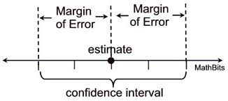
The margin of error (ME) quantifies the maximum expected difference between the sample estimate and the true population difference at a given confidence level.
![]()
Formula:
\( ME = t^* \cdot \sqrt{\dfrac{s_1^2}{n_1} + \dfrac{s_2^2}{n_2}} \)
- \(s_1, s_2\) = sample standard deviations
- \(n_1, n_2\) = sample sizes
- \(t^*\) = critical t-value for the desired confidence level with appropriate degrees of freedom (can use Satterthwaite approximation)
Interpretation: The margin of error is added and subtracted from the point estimate (\(\bar{x}_1 – \bar{x}_2\)) to form the confidence interval. It represents the range within which we expect the true difference of population means to lie with a specified level of confidence.
Example
Two teaching methods are compared. Sample 1: \(n_1 = 20\), \(\bar{x}_1 = 85\), \(s_1 = 5\). Sample 2: \(n_2 = 18\), \(\bar{x}_2 = 80\), \(s_2 = 6\). Construct the margin of error for a 95% confidence interval for \(\mu_1 – \mu_2\).
▶️ Answer / Explanation
Step 1: Determine standard error:
\( SE = \sqrt{\dfrac{5^2}{20} + \dfrac{6^2}{18}} = \sqrt{1.25 + 2} = \sqrt{3.25} \approx 1.803 \)
Step 2: Find \(t^*\) for 95% confidence (df ≈ 34): \(t^* \approx 2.032\)
Step 3: Compute margin of error:
\( ME = 2.032 \cdot 1.803 \approx 3.66 \)
Conclusion: The margin of error is approximately 3.66. The 95% confidence interval will be \( (\bar{x}_1 – \bar{x}_2) \pm 3.66 = 5 \pm 3.66 = [1.34, 8.66] \).
Confidence Interval Procedure for a Difference of Two Population Means (Unknown \(\sigma\))
When comparing two independent populations with unknown population standard deviations, the appropriate procedure is a two-sample t-interval for the difference of means, \(\mu_1 – \mu_2\).
Conditions:
- Randomness / Independence: Each sample should be collected randomly or through a randomized experiment. Samples must be independent of each other.
- Normality / Shape: Each population should be approximately normal, or the sample sizes should be large enough (\(n \ge 30\)) for the Central Limit Theorem to apply.
- Unknown population standard deviations: Use sample standard deviations \(s_1\) and \(s_2\) in place of \(\sigma_1\) and \(\sigma_2\).
Confidence interval formula:
\( (\bar{x}_1 – \bar{x}_2) \pm t^* \sqrt{\dfrac{s_1^2}{n_1} + \dfrac{s_2^2}{n_2}} \)
- \(\bar{x}_1, \bar{x}_2\) = sample means
- \(s_1, s_2\) = sample standard deviations
- \(n_1, n_2\) = sample sizes
- \(t^*\) = critical value from t-distribution (with appropriate degrees of freedom)
Example
A researcher wants to compare the average test scores of students from two different teaching methods. Sample 1: \(n_1 = 20\), \(\bar{x}_1 = 85\), \(s_1 = 5\). Sample 2: \(n_2 = 18\), \(\bar{x}_2 = 80\), \(s_2 = 6\). Construct a 95% confidence interval for \(\mu_1 – \mu_2\).
▶️ Answer / Explanation
Step 1: Identify point estimate:
\(\bar{x}_1 – \bar{x}_2 = 85 – 80 = 5\)
Step 2: Calculate standard error:
\( SE = \sqrt{\dfrac{5^2}{20} + \dfrac{6^2}{18}} = \sqrt{1.25 + 2} = \sqrt{3.25} \approx 1.803 \)
Step 3: Determine \(t^*\) (approx df ≈ 34) for 95% CI: \(t^* \approx 2.032\)
Step 4: Compute confidence interval:
\( 5 \pm 2.032 \times 1.803 \approx 5 \pm 3.66 \)
CI: \( 1.34 \text{ to } 8.66 \)
Interpretation: We are 95% confident that the mean score difference between teaching methods is between 1.34 and 8.66 points, with Method 1 higher on average.
