Home / AP Statistics 7.9 Carrying Out a Test for the Difference of Two Population Means Study Notes

AP Statistics 7.9 Carrying Out a Test for the Difference of Two Population Means Study Notes

AP Statistics 7.9 Carrying Out a Test for the Difference of Two Population Means Study Notes- New syllabus

AP Statistics 7.9 Carrying Out a Test for the Difference of Two Population Means Study Notes -As per latest AP Statistics Syllabus.

LEARNING OBJECTIVE

  • The t-distribution may be used to model variation.

Key Concepts:

  • Calculating the Test Statistic for a Difference of Two Population Means (\(\mu_1 – \mu_2\))
  • Interpreting the P-Value for a Difference of Two Population Means
  • Justifying a Claim About the Population Based on a Significance Test for a Difference of Two Population Means

AP Statistics -Concise Summary Notes- All Topics

Calculating the Test Statistic for a Difference of Two Population Means (\(\mu_1 - \mu_2\))

Calculating the Test Statistic for a Difference of Two Population Means (\(\mu_1 – \mu_2\))

To test hypotheses about the difference between two population means, we use a two-sample t-test statistic when population standard deviations are unknown.

Test statistic formula:

\( t = \dfrac{(\bar{x}_1 – \bar{x}_2) – (\mu_1 – \mu_2)_0}{\sqrt{\dfrac{s_1^2}{n_1} + \dfrac{s_2^2}{n_2}}} \)

  • \(\bar{x}_1, \bar{x}_2\) = sample means
  • \(s_1, s_2\) = sample standard deviations
  • \(n_1, n_2\) = sample sizes
  • \((\mu_1 – \mu_2)_0\) = hypothesized difference under the null hypothesis (often 0)

Degrees of freedom:

  • Can be approximated using the smaller of \(n_1 – 1\) and \(n_2 – 1\), or calculated more precisely using the Welch-Satterthwaite equation.

Example

Two teaching methods are compared. Sample 1: n₁ = 25, \(\bar{x}_1 = 85\), s₁ = 5. Sample 2: n₂ = 28, \(\bar{x}_2 = 80\), s₂ = 6. Test \(H_0: \mu_1 – \mu_2 = 0\).

▶️ Answer / Explanation

Step 1: Compute standard error:

\( SE = \sqrt{\dfrac{5^2}{25} + \dfrac{6^2}{28}} = \sqrt{1 + 1.286} = \sqrt{2.286} \approx 1.512 \)

Step 2: Compute test statistic:

\( t = \dfrac{85 – 80 – 0}{1.512} = \dfrac{5}{1.512} \approx 3.31 \)

Step 3: Approximate degrees of freedom: min(25-1, 28-1) = 24

Step 4: Compare t-value to t-distribution to find p-value.

Conclusion: Large t-value indicates strong evidence against \(H_0\), suggesting Method 1 leads to higher mean scores.

Interpreting the P-Value for a Difference of Two Population Means

Interpreting the P-Value for a Difference of Two Population Means

The p-value is the probability of obtaining a test statistic as extreme or more extreme than the observed value, assuming the null hypothesis is true.

Important Points:

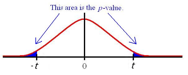
  • If the alternative hypothesis is two-sided (\(H_a: \mu_1 – \mu_2 \ne 0\)), the p-value is the probability of observing a t-value as far from 0 (in both directions) as the calculated t-statistic.
  • If the alternative is one-sided (\(H_a: \mu_1 – \mu_2 > 0\) or \(H_a: \mu_1 – \mu_2 < 0\)), the p-value is the probability of observing a t-value as extreme in the direction specified by the alternative.
  • A small p-value (typically ≤ α = 0.05) provides strong evidence against \(H_0\).
  • A large p-value suggests insufficient evidence to reject \(H_0\), but does not prove \(H_0\) is true.

Example

Using the previous two-sample example: t = 3.31, df = 24, testing \(H_0: \mu_1 – \mu_2 = 0\) vs \(H_a: \mu_1 – \mu_2 > 0\).

▶️ Answer / Explanation

Step 1: Determine p-value from t-distribution with df = 24.

Two-sided p-value ≈ 0.003; one-sided p-value ≈ 0.0015.

Step 2: Compare to α = 0.05 → p-value < α

Conclusion: The small p-value provides strong evidence against \(H_0\). There is convincing evidence that the mean score for Method 1 is higher than Method 2.

Justifying a Claim About the Population Based on a Significance Test for a Difference of Two Population Means

Justifying a Claim About the Population Based on a Significance Test for a Difference of Two Population Means

A significance test for a difference of two population means allows us to evaluate whether observed differences in sample means provide enough evidence to support a claim about the population.

Significance level (\(\alpha\)): Pre-determined threshold for rejecting the null hypothesis, commonly 0.05 or 0.01.

Decision rule:

    • If p-value ≤ α → reject \(H_0\), conclude evidence supports \(H_a\).
    • If p-value > α → fail to reject \(H_0\), conclude insufficient evidence to support \(H_a\).

Contextual conclusion: Always state the conclusion in terms of the populations and the research question.

  • Rejecting \(H_0\) does not prove \(H_0\) is false, it indicates sufficient evidence for the alternative hypothesis. Failing to reject \(H_0\) does not prove \(H_0\) is true, it indicates insufficient evidence for the alternative hypothesis.

Example

From previous example: Method 1 (n₁ = 25, x̄₁ = 85, s₁ = 5), Method 2 (n₂ = 28, x̄₂ = 80, s₂ = 6). Two-sample t-test: t = 3.31, df = 24, one-sided p-value ≈ 0.0015, α = 0.05.

▶️ Answer / Explanation

Step 1: Compare p-value to α → 0.0015 < 0.05 → reject \(H_0\).

Step 2: State conclusion in context → There is strong statistical evidence that the mean test score for students taught using Method 1 is higher than for those taught using Method 2.

Step 3: Emphasize reasoning → The small p-value indicates the observed difference would be very unlikely if the population means were equal. Therefore, the data provide sufficient evidence to support the claim in the research context.

Example

A nutritionist wants to test whether a new diet increases average weight loss compared to a standard diet. Sample 1 (new diet): n₁ = 30, x̄₁ = 7.2 kg, s₁ = 1.5 kg. Sample 2 (standard diet): n₂ = 32, x̄₂ = 5.8 kg, s₂ = 1.6 kg. Two-sample t-test: t ≈ 3.0, df ≈ 60, two-sided p-value ≈ 0.004, α = 0.05.

▶️ Answer / Explanation

Step 1: Compare p-value to α → 0.004 < 0.05 → reject \(H_0\).

Step 2: State conclusion in context → There is strong statistical evidence that participants on the new diet lose more weight on average than participants on the standard diet.

Step 3: Reasoning → The small p-value indicates that the observed difference in sample means would be very unlikely if there were no true difference in population means. Therefore, the claim that the new diet leads to greater weight loss is supported.

Scroll to Top