Home / AP Statistics 8.1 Introducing Statistics: Are My Results Unexpected? Study Notes

AP Statistics 8.1 Introducing Statistics: Are My Results Unexpected? Study Notes

AP Statistics 8.1 Introducing Statistics: Are My Results Unexpected? Study Notes- New syllabus

AP Statistics 8.1 Introducing Statistics: Are My Results Unexpected? Study Notes -As per latest AP Statistics Syllabus.

LEARNING OBJECTIVE

  • Given that variation may be random or not, conclusions are uncertain.

Key Concepts:

  • Introducing Statistics: Are My Results Unexpected?
  • Chi-Square Distributions
  • Null and Alternative Hypotheses for a Categorical Distribution
  • Testing a Distribution of Proportions in Categorical Data
  • Calculating Expected Counts for a Chi-Square Goodness-of-Fit Test
  • Conditions for a Chi-Square Goodness-of-Fit Test

AP Statistics -Concise Summary Notes- All Topics

Introducing Statistics: Are My Results Unexpected?

Introducing Statistics: Are My Results Unexpected?

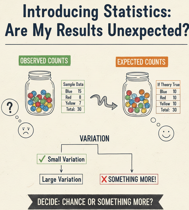
When analyzing categorical data, we often compare what we actually observe in a sample (observed counts) to what we would expect if a certain claim, theory, or model were true (expected counts). Variation between the observed and expected counts can help us decide whether results are consistent with chance variation or whether they suggest something more than random fluctuation.

Key Question:

Is the difference between the observed counts and the expected counts too large to be explained by chance alone?

Ideas suggested by variation:

  • Are the differences between observed and expected counts due to random sampling variability?
  • Do the results provide evidence that the actual distribution of the categorical variable is different from what was assumed?
  • Is there an association or effect present that makes the observed data inconsistent with the expected model?

Important Note:

Variation between what we find (observed counts) and what we expect to find (expected counts) may be due to random chance, but if the variation is unusually large, this may suggest that the model or assumption used to generate the expected counts is not correct.

Example 

A teacher expects that in her class of 30 students, 10 will prefer math, 10 will prefer science, and 10 will prefer history. After a survey, the observed counts are:

  • Math: 8
  • Science: 12
  • History: 10

Does the variation between the observed and expected counts suggest anything unexpected?

▶️ Answer / Explanation

The expected counts were all 10. The observed counts show small differences (Math: -2, Science: +2, History: 0). These variations could plausibly be due to random chance. The differences are minor and do not necessarily indicate a pattern or problem with the initial expectation.

Conclusion: The variation between observed and expected counts may be random; nothing in the data strongly suggests an unexpected result.

Example 

A survey expects that 25% of respondents prefer apples, 25% prefer bananas, 25% prefer oranges, and 25% prefer grapes. In a survey of 80 people, the observed counts are:

  • Apples: 18
  • Bananas: 22
  • Oranges: 20
  • Grapes: 20

 Does the observed variation from the expected counts suggest anything unusual?

▶️ Answer / Explanation

The expected counts for each fruit are \(80 \times 0.25 = 20\). The observed counts differ by -2, +2, 0, 0. These small differences are likely due to random variation in the sample. There is no strong evidence from these numbers alone to suggest that the population preference differs from the expected 25% for each fruit.

Conclusion: The variation observed is minor and can reasonably occur by chance; the results are not unexpectedly different from the expectations.

Chi-Square Distributions

Chi-Square Distributions

 A chi-square (\(\chi^2\)) distribution is a probability distribution that describes the distribution of a sum of the squares of independent standard normal random variables. It is commonly used to model the variation between observed and expected counts in categorical data.

Key Features:

  • The chi-square distribution is always non-negative (\(\chi^2 \ge 0\)) because it is based on squared values.
  • It is right-skewed, but the skew decreases as the degrees of freedom increase.
  • The shape of the chi-square distribution depends on the degrees of freedom (df).
    • Fewer degrees of freedom → more skewed.
    • More degrees of freedom → more symmetric and bell-shaped.
  • The mean of a chi-square distribution is equal to the degrees of freedom: \(\mu = df\).
  • The variance is \( \sigma^2 = 2 \cdot df \).

Applications in Statistics:

  • Goodness-of-fit tests: Comparing observed counts to expected counts for a single categorical variable.
  • Tests of independence: Determining whether two categorical variables are associated in a contingency table.
  • Homogeneity tests: Comparing distributions across multiple populations.

Example:

If we have 5 categories for a categorical variable, and we calculate the sum of squared differences between observed and expected counts divided by expected counts, that sum follows a chi-square distribution with \(df = 5 – 1 = 4\).

Example 

A small company wants to see if the distribution of employees across four departments matches what they expect based on company policy. Expected distribution: 25% in each department. There are 40 employees:

  • Observed counts: Department A = 8, B = 12, C = 10, D = 10
  • Expected counts: 40 × 0.25 = 10 per department

 Describe the chi-square distribution that would be used to assess whether the observed counts differ from expected counts.

▶️ Answer / Explanation

Step 1 — Degrees of freedom

For a goodness-of-fit test with \(k = 4\) categories: \(\displaystyle df = k – 1 = 4 – 1 = 3.\)

Step 2 — Shape of the distribution

  • The chi-square distribution is right-skewed because \(df = 3\) is small.
  • It starts at 0 on the horizontal axis and has a long tail to the right.
  • The mean is \(\mu = df = 3\) and variance \(\sigma^2 = 2 \cdot df = 6\).

Step 3 — Interpretation

If we compute the chi-square statistic for the observed vs. expected counts:

\(\displaystyle \chi^2 = \sum \dfrac{(O_i – E_i)^2}{E_i} = \dfrac{(8-10)^2}{10} + \dfrac{(12-10)^2}{10} + \dfrac{(10-10)^2}{10} + \dfrac{(10-10)^2}{10} = 0.8\)

This value would be compared to the chi-square distribution with \(df = 3\) to determine if the observed variation is unexpectedly large. In this case, the variation is small and consistent with random chance.

Null and Alternative Hypotheses for a Categorical Distribution

Null and Alternative Hypotheses for a Categorical Distribution

When testing whether a categorical variable follows a specified distribution of proportions, we define hypotheses as follows:

Null hypothesis (\(H_0\)): The observed categorical data follow the specified distribution.

Example: \(H_0:\) The proportions of students in each grade (freshman, sophomore, junior, senior) are 25%, 25%, 25%, 25%.

Alternative hypothesis (\(H_a\)): The observed categorical data do not follow the specified distribution.

Example: \(H_a:\) The proportions of students in the grades are not all equal to 25%.

Key Points:

  • The null hypothesis is often stated with exact proportions based on theoretical expectations or claims.
  • The alternative hypothesis is non-directional (two-sided), indicating that the observed distribution differs in at least one category.
  • This setup is used in goodness-of-fit tests, where the goal is to compare observed counts to expected counts under \(H_0\).

Example : A candy company claims that their 4-color candy pack contains equal numbers of red, green, blue, and yellow candies.

\(H_0:\) Proportions are 25% each. 

\(H_a:\) At least one color’s proportion is different from 25%.

Example 

A school claims that students’ favorite lunch choices are equally distributed among four options: Pizza, Sandwich, Salad, and Pasta. A survey of 80 students yields the following observed counts:

  • Pizza: 22
  • Sandwich: 18
  • Salad: 20
  • Pasta: 20

Identify the null and alternative hypotheses for testing if the observed counts match the expected distribution.

▶️ Answer / Explanation

Step 1 — Define null hypothesis (\(H_0\))

\(H_0:\) The proportions of students choosing each lunch option are equal, i.e., 25% for Pizza, 25% for Sandwich, 25% for Salad, and 25% for Pasta.

Step 2 — Define alternative hypothesis (\(H_a\))

\(H_a:\) At least one lunch option has a proportion different from 25%. In other words, the observed distribution of favorite lunch choices does not match the claimed equal distribution.

Step 3 — Contextual interpretation

If we proceed with a goodness-of-fit test, we will compare the observed counts to expected counts (80 × 0.25 = 20 for each option). The hypotheses guide the test and help determine if the differences are due to random variation or indicate a real discrepancy from the claimed distribution.

Testing a Distribution of Proportions in Categorical Data

Testing a Distribution of Proportions in Categorical Data

 We want to determine whether observed counts in categorical data match a claimed or expected distribution of proportions.

Appropriate Testing Method:

Goodness-of-Fit Test using the Chi-Square (\(\chi^2\)) statistic

  • Used when:
    • There is one categorical variable with \(k\) categories.
    • We have specified expected proportions for each category under a null hypothesis \(H_0\).
    • We want to compare observed counts to expected counts to see if deviations are larger than can be explained by random chance.

Steps for the Test:

  1. Define the null hypothesis \(H_0\): The observed proportions match the expected proportions.
  2. Define the alternative hypothesis \(H_a\): At least one category has a proportion different from the expected.
  3. Calculate expected counts: \(E_i = N \times \text{expected proportion}_i\), where \(N\) is total sample size.
  4. Compute the chi-square statistic: \(\displaystyle \chi^2 = \sum_{i=1}^k \dfrac{(O_i – E_i)^2}{E_i}\), where \(O_i\) is the observed count.
  5. Determine degrees of freedom: \(df = k – 1\).
  6. Compare the statistic to the \(\chi^2\) distribution with \(df\) to calculate a p-value and draw a conclusion.

Notes:

  • This method assesses whether the observed variation in counts is unusually large compared to what we would expect under the null hypothesis.
  • It is suitable for any categorical variable with two or more categories, as long as expected counts are sufficiently large (usually ≥5 for each category).

Example 

A toy company claims that their four-color candy packs contain equal numbers of red, green, blue, and yellow candies. A random sample of 80 candies yields the following counts:

  • Red: 18
  • Green: 22
  • Blue: 20
  • Yellow: 20

What is the appropriate test to determine if the observed distribution of candy colors matches the company’s claim?

▶️ Answer / Explanation

Step 1 — Identify the test

The appropriate test is a chi-square goodness-of-fit test, because we are comparing observed counts in one categorical variable (candy color) to expected counts based on specified proportions (25% each color).

Step 2 — Expected counts

Expected count for each color: \(E = 80 \times 0.25 = 20\).

Step 3 — Interpretation

The chi-square test would compare the observed counts (18, 22, 20, 20) to the expected counts (20, 20, 20, 20) to see if the differences are unusually large. This determines whether the observed variation could plausibly be due to random chance or indicates a departure from the claimed distribution.

Calculating Expected Counts for a Chi-Square Goodness-of-Fit Test

Calculating Expected Counts for a Chi-Square Goodness-of-Fit Test

 Expected counts are the counts we would anticipate in each category if the null hypothesis \(H_0\) is true. They provide the baseline to compare with observed counts.

Formula:

\(\displaystyle E_i = N \times p_i\)

  • \(E_i\) = expected count for category \(i\)
  • \(N\) = total sample size
  • \(p_i\) = hypothesized proportion for category \(i\) under \(H_0\)

Key Points:

  • All expected counts should generally be at least 5 for the chi-square test to be valid.
  • Expected counts are calculated before comparing to observed counts.
  • They reflect the distribution claimed by the null hypothesis, not the actual data.

Example 

A school claims that students’ favorite subjects are equally distributed among Math, Science, English, and History. A survey of 60 students yields observed counts:

  • Math: 14
  • Science: 18
  • English: 16
  • History: 12

Calculate the expected counts for each subject under the null hypothesis that all subjects are equally preferred.

▶️ Answer / Explanation

Step 1 — Identify total sample size

Total students: \(N = 60\).

Step 2 — Hypothesized proportions

Equal preference implies \(p_i = 0.25\) for each subject.

Step 3 — Calculate expected counts

  • Math: \(E = 60 \times 0.25 = 15\)
  • Science: \(E = 60 \times 0.25 = 15\)
  • English: \(E = 60 \times 0.25 = 15\)
  • History: \(E = 60 \times 0.25 = 15\)

Step 4 — Interpretation

These expected counts (15 for each subject) are what we would expect if students truly have no preference. Observed counts can now be compared to these expected counts to assess whether the variation is larger than expected by chance.

Conditions for a Chi-Square Goodness-of-Fit Test

Conditions for a Chi-Square Goodness-of-Fit Test

Before performing a chi-square test for goodness-of-fit, we must verify that the data meet the necessary conditions to ensure valid inferences:

1. Random: The data come from a random sample or a randomized experiment.

This ensures that the sample is representative of the population.

2. Expected Counts (Large Enough Sample): Each expected count \(E_i\) should generally be at least 5.

This ensures that the chi-square approximation to the sampling distribution is valid.

3. Independence: The observations must be independent of each other.

If sampling without replacement, the 10% condition should be satisfied: \(n \le 0.1N\), where \(N\) is the population size.

Notes:

  • If any expected count is less than 5, consider combining categories or using a different test.
  • Randomness, independence, and sufficiently large expected counts together ensure that the chi-square test statistic follows the chi-square distribution approximately under the null hypothesis.

Example 

A candy company claims that their four-color candy packs contain equal numbers of red, green, blue, and yellow candies. A sample of 80 candies yields:

  • Observed: Red = 18, Green = 22, Blue = 20, Yellow = 20
  • Expected (if proportions are equal): 20 each

Verify that conditions are met for a chi-square goodness-of-fit test.

▶️ Answer / Explanation

Step 1 — Random: The sample is assumed to be randomly selected from the candy packs. 

Step 2 — Expected counts: Each expected count \(E_i = 80 \times 0.25 = 20\). All expected counts ≥ 5. 

Step 3 — Independence: Each candy is counted independently, and the sample size is much smaller than the total population of candies (satisfies 10% condition). 

Conclusion: All conditions are satisfied. It is appropriate to proceed with the chi-square goodness-of-fit test to evaluate whether the observed counts differ from the expected distribution.

Scroll to Top