AP Statistics 8.3 Carrying Out a Chi-Square Test for Goodness of Fit Study Notes
AP Statistics 8.3 Carrying Out a Chi-Square Test for Goodness of Fit Test Study Notes- New syllabus
AP Statistics 8.3 Carrying Out a Chi-Square Test for Goodness of Fit Test Study Notes -As per latest AP Statistics Syllabus.
LEARNING OBJECTIVE
- The chi-square distribution may be used to model variation.
Key Concepts:
- Chi-Square Test Statistic for Goodness-of-Fit
- P-Value for Chi-Square Goodness-of-Fit Test
- Justifying a Claim Based on a Chi-Square Goodness-of-Fit Test
Chi-Square Test Statistic for Goodness-of-Fit
The chi-square test statistic measures how far the observed counts are from the expected counts under the null hypothesis. The larger the differences, the more evidence against \(H_0\).
Formula:
\(\displaystyle \chi^2 = \sum_{i=1}^k \frac{(O_i – E_i)^2}{E_i}\)
- \(O_i\) = observed count for category \(i\)
- \(E_i\) = expected count for category \(i\) under \(H_0\)
- \(k\) = number of categories
Key Points:
- Each term \((O_i – E_i)^2 / E_i\) measures the squared difference between observed and expected counts, scaled by the expected count.
- The sum of these terms gives the test statistic \(\chi^2\), which is compared to a chi-square distribution with \(df = k – 1\) degrees of freedom for goodness-of-fit tests.
Example
A school claims that students’ favorite subjects are equally preferred among Math, Science, English, and History. A survey of 60 students gives observed counts:
- Math: 14
- Science: 18
- English: 16
- History: 12
Expected counts under \(H_0\) (equal preference): 60 × 0.25 = 15 for each subject.
Calculate the chi-square test statistic.
▶️ Answer / Explanation
Step 1 — Apply the formula:
\(\displaystyle \chi^2 = \sum \frac{(O_i – E_i)^2}{E_i}\)
Step 2 — Calculate each term:
- Math: \((14 – 15)^2 / 15 = 1 / 15 \approx 0.067\)
- Science: \((18 – 15)^2 / 15 = 9 / 15 = 0.6\)
- English: \((16 – 15)^2 / 15 = 1 / 15 \approx 0.067\)
- History: \((12 – 15)^2 / 15 = 9 / 15 = 0.6\)
Step 3 — Sum the terms:
\(\chi^2 \approx 0.067 + 0.6 + 0.067 + 0.6 = 1.334\)
Step 4 — Interpretation: The chi-square statistic of 1.334 measures how much the observed counts differ from expected counts. This value can now be compared to a chi-square distribution with \(df = k – 1 = 4 – 1 = 3\) to determine if the difference is statistically significant.
P-Value for Chi-Square Goodness-of-Fit Test
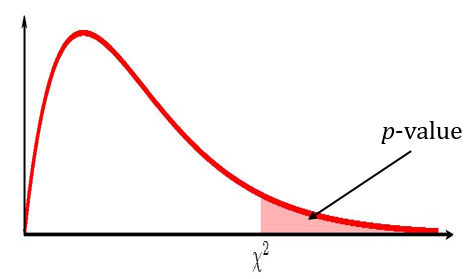
The p-value is the probability of obtaining a chi-square test statistic as extreme or more extreme than the observed value, assuming the null hypothesis is true.
Steps to Determine the p-value:
- Calculate the chi-square test statistic: \(\chi^2 = \sum \dfrac{(O_i – E_i)^2}{E_i}\).
- Determine the degrees of freedom: \(df = k – 1\), where \(k\) is the number of categories.
- Use the chi-square distribution with \(df\) to find the probability that \(\chi^2 \ge \chi^2_\text{observed}\).
Interpreting the p-value:
- Small p-value (\(p \le \alpha\)) → Observed differences are unlikely under \(H_0\); reject \(H_0\).
- Large p-value (\(p > \alpha\)) → Observed differences are plausible under \(H_0\); fail to reject \(H_0\).
- The p-value does not measure the probability that \(H_0\) is true; it measures the probability of observing data at least as extreme assuming \(H_0\) is true.
Example
Recall the previous example: A survey of 60 students on favorite subjects gave observed counts:
- Math: 14, Science: 18, English: 16, History: 12
Expected counts: 15 each. Chi-square test statistic: \(\chi^2 = 1.334\) with \(df = 3\).
Determine and interpret the p-value for the chi-square test.
▶️ Answer / Explanation
Step 1 — Use the chi-square distribution:
We calculate \(P(\chi^2 \ge 1.334)\) using a chi-square table or software with \(df = 3\).
Step 2 — Find the p-value:
From the chi-square table, for \(\chi^2 = 1.334\) and \(df = 3\), the p-value ≈ 0.72.
Step 3 — Interpret the p-value:
- The p-value is large (0.72 > typical \(\alpha = 0.05\)), so the observed differences could easily occur by random chance.
- Fail to reject \(H_0\): There is no strong evidence that students’ preferences differ from equal proportions.
- This means the observed variation is consistent with the claimed distribution.
Justifying a Claim Based on a Chi-Square Goodness-of-Fit Test
A chi-square goodness-of-fit test allows us to assess whether observed categorical data are consistent with a claimed distribution. The results can be used to justify or refute a claim about the population proportions.
Steps for Justifying a Claim:
- State hypotheses:
- \(H_0\): The population proportions are as claimed.
- \(H_a\): At least one population proportion differs from the claim.
- Check conditions: Random sample, independent observations, and expected counts ≥ 5.
- Calculate the chi-square statistic: \(\displaystyle \chi^2 = \sum \frac{(O_i – E_i)^2}{E_i}\).
- Determine the p-value: Find \(P(\chi^2 \ge \chi^2_\text{observed})\) using the chi-square distribution with \(df = k – 1\).
- Compare p-value to significance level (\(\alpha\)):
- If \(p \le \alpha\): Reject \(H_0\). There is sufficient evidence to conclude that the population does not match the claimed distribution.
- If \(p > \alpha\): Fail to reject \(H_0\). There is insufficient evidence to refute the claim; observed variation could be due to chance.
- Contextual interpretation: Always state the conclusion in terms of the population and the claim.
Notes:
- The chi-square test does not prove that the null hypothesis is true; it only assesses whether the observed data are consistent with the claimed distribution.
- A small p-value provides strong evidence against the claim, while a large p-value indicates that the claim is plausible.
Example
A candy company claims that its four-color candy packs contain equal numbers of red, green, blue, and yellow candies. A random sample of 80 candies yields:
- Red: 18
- Green: 22
- Blue: 20
- Yellow: 20
Chi-square statistic: \(\chi^2 = 0.8\), \(df = 3\), p-value ≈ 0.85.
Can we justify the company’s claim about equal proportions of candy colors?
▶️ Answer / Explanation
Step 1 — Compare p-value to significance level:
Assume \(\alpha = 0.05\). The p-value (0.85) is much larger than 0.05.
Step 2 — Decision: Fail to reject \(H_0\).
Step 3 — Contextual interpretation:
There is insufficient evidence to conclude that the proportions of candy colors differ from equal. The observed variation is consistent with random chance. Therefore, the company’s claim about equal proportions is justified based on this sample.