Determine the P-Value for a Chi-Square Significance Test for Independence or Homogeneity
The p-value represents the probability of obtaining a chi-square statistic as extreme or more extreme than the observed value, assuming the null hypothesis is true.
- The p-value is found using the chi-square distribution with the appropriate degrees of freedom.
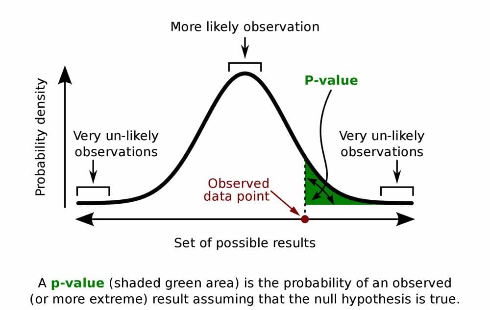
- It tells us how surprising the observed data are if the null hypothesis \( H_0 \) (no association or no difference) were true.
Steps to Determine the P-Value:
- Calculate the Chi-Square Statistic:
\( \displaystyle \chi^2 = \sum \dfrac{(O_{ij} – E_{ij})^2}{E_{ij}} \) - Determine Degrees of Freedom:
\( df = (\text{number of rows} – 1)(\text{number of columns} – 1) \) - Find the P-Value:
Use a chi-square distribution table or statistical software to find the probability \( P(\chi^2 \ge \text{observed value}) \).
Key Notes:
- The p-value assumes \( H_0 \) is true.
- Larger values of \( \chi^2 \) → smaller p-values (stronger evidence against \( H_0 \)).
Example:
A study of snack preference by gender among 100 students produced a chi-square statistic of \( \chi^2 = 16.66 \) with \( df = 1 \).
Determine the p-value.
▶️ Answer / Explanation
Step 1 — Find P-Value:
Using the chi-square distribution with \( df = 1 \), \( P(\chi^2 \ge 16.66) ≈ 0.00004 \).
Step 2 — Interpretation:
The probability of observing such an extreme chi-square value if \( H_0 \) is true is extremely small (0.00004).
Conclusion:
This very small p-value indicates that the observed data are highly inconsistent with the null hypothesis.