Home / AP Statistics 9.2 Confidence Intervals for the Slope of a Regression Model Study Notes

AP Statistics 9.2 Confidence Intervals for the Slope of a Regression Model Study Notes

AP Statistics 9.2 Confidence Intervals for the Slope of a Regression Model Study Notes- New syllabus

AP Statistics 9.2 Confidence Intervals for the Slope of a Regression Model Study Notes -As per latest AP Statistics Syllabus.

LEARNING OBJECTIVE

  • An interval of values should be used to estimate parameters, in order to account for uncertainty

Key Concepts:

  • Regression Inference: Residuals and Sampling Distribution of the Slope
  • Verifying Conditions for a Confidence Interval for the Slope (\(\beta\))
  • Margin of Error for the Slope (\(\beta\)) in Regression
  • Confidence Interval for the Slope (\(\beta\)) of a Regression Model

AP Statistics -Concise Summary Notes- All Topics

Regression Inference: Residuals and Sampling Distribution of the Slope

Regression Inference: Residuals and Sampling Distribution of the Slope

Population vs. Sample Regression Lines:

  • The population regression line is given by: \( \mu_y = \alpha + \beta x \).
  • The sample regression line is estimated from data: \( \hat{y} = a + bx \), where \( a \) and \( b \) are the least-squares estimates of \( \alpha \) and \( \beta \).

Residuals:

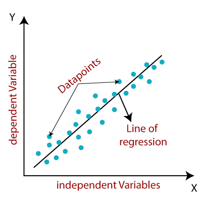
For each observation \((x_i, y_i)\), the residual is:

\( e_i = y_i – \hat{y}_i = y_i – (a + b x_i) \).

  • This residual estimates the difference between the observed response and the true population regression line deviation: \( y_i – (\alpha + \beta x_i) \).

Standard Deviation of Residuals (s):

In the population, the variability around the regression line is measured by \( \sigma \), the standard deviation of deviations from the line.

  • In the sample, we estimate \( \sigma \) with the standard deviation of the residuals:

\( s = \sqrt{\dfrac{\sum (y_i – \hat{y}_i)^2}{n – 2}} \).

  • Why \( n-2 \)? We lose 2 degrees of freedom because both slope (\( b \)) and intercept (\( a \)) are estimated from the data before calculating predicted values.

Sampling Distribution of the Slope (b):

The slope \( b \) of the sample regression line varies from sample to sample.

Mean: The mean of the sampling distribution of \( b \) equals the population slope:

\( \mu_b = \beta \).

Standard deviation: The spread of the sampling distribution of \( b \) is given by:

\( \sigma_b = \dfrac{\sigma}{\sqrt{\sum (x_i – \bar{x})^2}} \).

  • Since \( \sigma \) is usually unknown, we estimate it using the residual standard deviation \( s \).

Interpretation:

The sampling distribution of \( b \) tells us how much the estimated slope is expected to vary from sample to sample due to random sampling. A smaller \( \sigma_b \) means more precise estimates of the slope.

Example 

A study examines how weekly study hours (x) relate to exam score (y). A simple random sample of n = 10 students is collected and a least-squares line is fitted. The regression output (summary values) gives:

  • Estimated slope: \(b = 2.50\).
  • Sum of squared deviations of \(x\) about its mean: \(\displaystyle \sum (x_i – \bar{x})^2 = SS_x = 82.5\).
  • Sum of squared residuals (SSE): \(\displaystyle \sum (y_i – \hat{y}_i)^2 = 140.76\).

Use these values to

(a) estimate the standard deviation of the sampling distribution of \(b\), and

(b) compute the test statistic for \(H_0:\; \beta = 0\).

▶️ Answer / Explanation

Step 1 — Estimate the residual standard deviation \(s\)

The residual standard deviation is

\( s = \sqrt{\dfrac{\sum (y_i – \hat{y}_i)^2}{\,n-2\,}} = \sqrt{\dfrac{140.76}{10-2}} = \sqrt{\dfrac{140.76}{8}} \).

Calculate:

\( s = \sqrt{17.595} \approx 4.20. \)

Step 2 — Estimate the standard deviation (standard error) of \(b\)

The standard deviation (standard error) of the sampling distribution of \(b\) is estimated by

\( SE_b = \dfrac{s}{\sqrt{\sum (x_i – \bar{x})^2}} = \dfrac{s}{\sqrt{SS_x}}. \)

Plug in values:

\( SE_b \approx \dfrac{4.20}{\sqrt{82.5}} = \dfrac{4.20}{9.082} \approx 0.463. \)

Interpretation of \(SE_b\):

This means that repeated samples of size 10 from the same population would produce slope estimates \(b\) with a typical variation of about \(0.463\) around the true slope \(\beta\).

Step 3 — Test statistic for \(H_0:\; \beta = 0\)

The t-statistic is

\( t = \dfrac{b – 0}{SE_b} = \dfrac{2.50}{0.463} \approx 5.40. \)

Degrees of freedom: \( df = n – 2 = 8.\)

Step 4 — Conclusion (brief)

A t value of about \(5.40\) with \(8\) df gives a very small p-value (much less than 0.01), so we have strong evidence to reject \(H_0:\; \beta=0\). In context: there is strong evidence that study hours are positively associated with exam score (the population slope \(\beta\) is greater than 0).

Summary of numeric results:

  • Residual SD: \( s \approx 4.20\).
  • Estimated standard error of slope: \( SE_b \approx 0.463\).
  • Test statistic: \( t \approx 5.40 \) with \(df = 8\) → very small p-value → reject \(H_0\).

Verifying Conditions for a Confidence Interval for the Slope (\(\beta\))

Verifying Conditions for a Confidence Interval for the Slope (\(\beta\))

Before calculating a confidence interval for the slope of a regression line, certain conditions must be checked to ensure valid inference.

Conditions:

Linearity: The relationship between the explanatory variable (\(x\)) and the response variable (\(y\)) should be approximately linear.

  • Check using a scatter plot or residual plot (residuals should not show curvature).

Independent observations: Each data point should be independent of the others.

  • Random sampling or randomized experiment is required.
  • If data are collected over time or in clusters, independence must be considered carefully.

Normality of residuals: For a fixed \(x\), the residuals (\(y_i – \hat{y}_i\)) should be approximately normally distributed.

  • Check using a histogram, normal probability plot, or residual plot.

Equal variance (Homoscedasticity): The spread of residuals should be roughly constant across all values of \(x\).

  • Residual plot should show no funneling or fanning.

Notes:

These conditions are sometimes summarized as LINE: Linearity, Independence, Normality, Equal variance.

If conditions are met, the standard error of the slope (\(SE_b\)) can be used to calculate a confidence interval for the population slope (\(\beta\)):

\( \text{CI: } b \pm t^* \cdot SE_b \), where \( t^* \) comes from the t-distribution with \( df = n-2 \).

Example 

A researcher studies how weekly exercise hours (\(x\)) affect resting heart rate (\(y\)) in 12 adults. The sample regression line is found to be \(\hat{y} = 80 – 1.5x\).

Summary statistics from the sample:

  • Residual standard deviation: \( s = 3.0 \)
  • Sum of squared deviations of \(x\): \(\sum (x_i – \bar{x})^2 = 40\)
  • Sample size: \( n = 12 \)

Construct a 95% confidence interval for the population slope \(\beta\), and verify that conditions for inference are reasonable.

▶️ Answer / Explanation

Step 1 — Verify conditions:

  • Linearity: Scatter plot shows roughly a straight-line downward trend → condition met 
  • Independence: Data collected from a simple random sample → condition met 
  • Normality: Residuals histogram and normal probability plot approximately normal → condition met 
  • Equal variance: Residual plot shows roughly constant spread → condition met 

Step 2 — Compute standard error of the slope:

\( SE_b = \dfrac{s}{\sqrt{\sum (x_i – \bar{x})^2}} = \dfrac{3.0}{\sqrt{40}} = \dfrac{3.0}{6.3246} \approx 0.474 \)

Step 3 — Find t* for 95% CI:

Degrees of freedom: \( df = n – 2 = 12 – 2 = 10 \)

From t-table, \( t^*_{0.975,10} \approx 2.228 \)

Step 4 — Construct confidence interval:

\( b \pm t^* \cdot SE_b = -1.5 \pm 2.228 \cdot 0.474 \) \( -1.5 \pm 1.056 \)
95% CI: \( (-2.556, -0.444) \)

Step 5 — Interpretation:

We are 95% confident that for each additional hour of weekly exercise, the population resting heart rate decreases by between 0.444 and 2.556 beats per minute.

Margin of Error for the Slope (\(\beta\)) in Regression

Margin of Error for the Slope (\(\beta\)) in Regression

The margin of error (ME) for a confidence interval for the slope of a regression line quantifies the range around the sample slope (\(b\)) within which we are confident the true population slope (\(\beta\)) lies.

Formula:

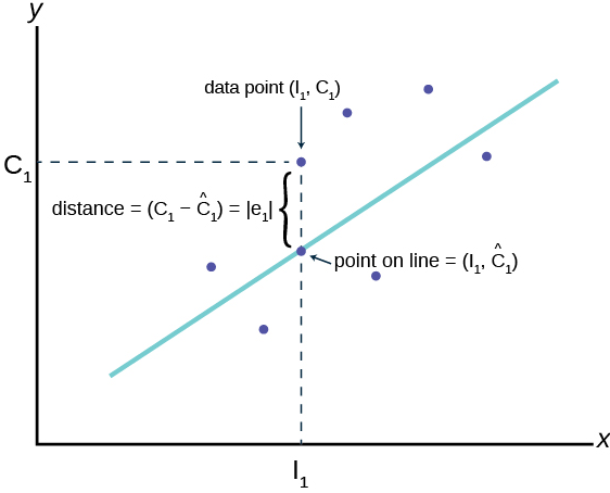
\( \text{ME} = t^* \cdot SE_b \)

  • \( t^* \) = critical value from the t-distribution with \( df = n – 2 \), based on the desired confidence level (e.g., 95%).

\( SE_b \) = standard error of the slope, computed as:

  • \( SE_b = \dfrac{s}{\sqrt{\sum (x_i – \bar{x})^2}} \)

where \( s \) = residual standard deviation, \( \sum (x_i – \bar{x})^2 \) = sum of squared deviations of \(x\) values about their mean.

Interpretation:

  • The margin of error is half the width of the confidence interval for the slope.
  • Smaller \( SE_b \) or lower \( t^* \) (smaller confidence level) → smaller margin of error → more precise estimate of slope.

Example 

A study examines the effect of hours of sleep per night (\(x\)) on reaction time (\(y\)) for a sample of 15 participants. The sample regression line is \(\hat{y} = 200 – 3.2x\).

Summary statistics:

  • Residual standard deviation: \( s = 5.0 \)
  • Sum of squared deviations of \(x\): \(\sum (x_i – \bar{x})^2 = 50\)
  • Sample size: \( n = 15 \)

Determine the margin of error for a 95% confidence interval for the population slope \(\beta\).

▶️ Answer / Explanation

Step 1 — Compute the standard error of the slope:

\( SE_b = \dfrac{s}{\sqrt{\sum (x_i – \bar{x})^2}} = \dfrac{5.0}{\sqrt{50}} = \dfrac{5.0}{7.071} \approx 0.707 \)

Step 2 — Determine t* for 95% confidence:

Degrees of freedom: \( df = n – 2 = 15 – 2 = 13 \)

From t-table, \( t^*_{0.975,13} \approx 2.160 \)

Step 3 — Compute margin of error:

\( \text{ME} = t^* \cdot SE_b = 2.160 \cdot 0.707 \approx 1.527 \)

Step 4 — Interpretation:

We are 95% confident that the sample slope \(b = -3.2\) is within ±1.527 of the true population slope \(\beta\). Therefore, the 95% confidence interval for \(\beta\) is approximately:

\( -3.2 \pm 1.527 \Rightarrow (-4.727, -1.673) \)

Confidence Interval for the Slope (\(\beta\)) of a Regression Model

Confidence Interval for the Slope (\(\beta\)) of a Regression Model

A confidence interval for the slope of a regression line estimates the range of plausible values for the population slope \(\beta\).

Formula:

\( \text{CI: } b \pm t^* \cdot SE_b \)

  • \( b \) = sample slope from least-squares regression line \( \hat{y} = a + bx \)
  • \( SE_b = \dfrac{s}{\sqrt{\sum (x_i – \bar{x})^2}} \), where \( s \) = residual standard deviation
  • \( t^* \) = critical value from the t-distribution with \( df = n – 2 \), based on the confidence level (e.g., 95%)

Interpretation:

  • We are $\rm C\%$ confident that the interval contains the true population slope \(\beta\).
  • The confidence interval quantifies the precision of the estimated slope \(b\).

Example 

A study investigates how weekly study hours (\(x\)) affect exam scores (\(y\)) in a sample of 10 students. The sample regression line is \(\hat{y} = 75 + 2.5x\).

Summary statistics:

  • Residual standard deviation: \( s = 4.2 \)
  • Sum of squared deviations of \(x\): \(\sum (x_i – \bar{x})^2 = 82.5\)
  • Sample size: \( n = 10 \)

Construct a 95% confidence interval for the population slope \(\beta\).

▶️ Answer / Explanation

Step 1 — Compute standard error of the slope:

\( SE_b = \dfrac{s}{\sqrt{\sum (x_i – \bar{x})^2}} = \dfrac{4.2}{\sqrt{82.5}} = \dfrac{4.2}{9.082} \approx 0.462 \)

Step 2 — Determine t* for 95% confidence:

Degrees of freedom: \( df = n – 2 = 10 – 2 = 8 \)

From t-table, \( t^*_{0.975,8} \approx 2.306 \)

Step 3 — Compute confidence interval:

\( \text{CI: } b \pm t^* \cdot SE_b = 2.5 \pm 2.306 \cdot 0.462 \) \( 2.5 \pm 1.066 \)
95% CI: \( (1.434, 3.566) \)

Step 4 — Interpretation:

We are 95% confident that for each additional hour of weekly study, the population mean exam score increases by between 1.434 and 3.566 points.

Scroll to Top