
Question
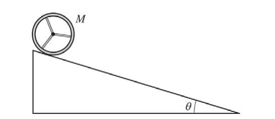
A wooden wheel of mass \(M\), consisting of a rim with spokes, rolls down a ramp that makes an angle \(\theta\) with the horizontal, as shown above. The ramp exerts a force of static friction on the wheel so that the wheel rolls without slipping.
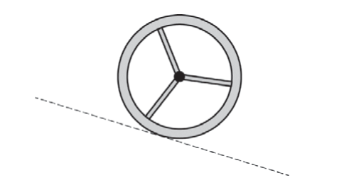
Most-appropriate topic codes (AP Physics \(1\)):
• Topic \(2.5\) — Newton’s Second Law (Part \( \mathrm{(b)} \), Part \( \mathrm{(c)(i)} \))
• Topic \(2.7\) — Kinetic and Static Friction (Part \( \mathrm{(a)} \), Part \( \mathrm{(b)} \), Part \( \mathrm{(c)} \))
• Topic \(3.3\) — Potential Energy (Part \( \mathrm{(c)(ii)} \))
• Topic \(3.4\) — Conservation of Energy (Part \( \mathrm{(c)(ii)} \))
• Topic \(5.3\) — Torque (Part \( \mathrm{(a)(ii)} \))
• Topic \(6.1\) — Rotational Kinetic Energy (Part \( \mathrm{(c)(ii)} \))
• Topic \(6.5\) — Rolling (Part \( \mathrm{(a)} \), Part \( \mathrm{(c)} \))
▶️ Answer/Explanation
(a)(i)
The force diagram should include \(3\) forces: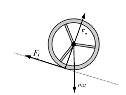
\(Mg\), the gravitational force, starting at the center of the wheel and directed vertically downward.
\(F_N\), the normal force, starting at the wheel-ramp contact point and directed perpendicular to the ramp, away from the surface.
\(F_f\), the static friction force, starting at the wheel-ramp contact point and directed up the ramp.
(a)(ii)
\(\boxed{\text{The friction force}}\)
Friction causes the change in angular velocity because it is the only force that produces a torque about the wheel’s center of mass. The gravitational force acts at the center of mass, so it has no lever arm about the center. The normal force points approximately through the center of the wheel, so it also produces no torque about the center.
Therefore, the static friction force provides the torque that increases the wheel’s angular speed as it rolls down the ramp.
(b)
Choose the positive direction to be down the ramp. The component of gravity down the ramp is
\(Mg\sin\theta\)
The friction force is directed up the ramp, opposite the wheel’s translational motion. The problem states that the friction force is \(40\%\) of the magnitude of the force component directed opposite friction, so
\(F_f=0.40Mg\sin\theta\)
Apply Newton’s second law along the ramp:
\(\sum F_{\parallel}=Ma\)
\(Mg\sin\theta-F_f=Ma\)
Substitute \(F_f=0.40Mg\sin\theta\):
\(Mg\sin\theta-0.40Mg\sin\theta=Ma\)
\(0.60Mg\sin\theta=Ma\)
Divide by \(M\):
\(\boxed{a=0.60g\sin\theta}\)
(c)(i)
\(\boxed{\text{Block}}\)
The block slides with negligible friction, so the only force component accelerating it down the ramp is \(Mg\sin\theta\). Thus, its acceleration is
\(a_{\text{block}}=g\sin\theta\)
The wheel has static friction directed up the ramp, so its net force down the ramp is smaller:
\(F_{\text{net,wheel}}=Mg\sin\theta-F_f\)
Therefore, the wheel has a smaller translational acceleration than the block. Since both start from rest and travel down the same ramp from the same height, the block reaches the bottom with the greater speed.
(c)(ii)
Both objects lose the same amount of gravitational potential energy because they have the same mass \(M\) and descend through the same vertical height.
For the block, essentially all of the lost gravitational potential energy becomes translational kinetic energy:
\(\Delta U_g \rightarrow K_{\text{trans}}\)
For the wheel, the lost gravitational potential energy becomes both translational kinetic energy and rotational kinetic energy:
\(\Delta U_g \rightarrow K_{\text{trans}}+K_{\text{rot}}\)
Since some of the wheel’s energy is rotational, less energy is available as translational kinetic energy compared with the block. Therefore, the block has the greater translational speed at the bottom.
Question
Most-appropriate topic codes (AP Physics 1):
• Topic 4.1 — Linear Momentum (Parts (a), (b))
• Topic 4.3 — Conservation of Linear Momentum (Parts (a), (b), (c))
• Topic 4.4 — Elastic and Inelastic Collisions (All parts)
• Topic 1.1 — Experimental Design and Data Analysis (Parts (a), (b), (c))
▶️ Answer/Explanation
(a)
A perfectly elastic collision is one in which both momentum and kinetic energy are conserved. To test whether a collision is elastic, one must compare the total mechanical energy before the collision to the total mechanical energy after the collision. For a ball bouncing off a hard floor, this reduces to comparing the speed (or a speed-related quantity such as drop height) just before and just after the bounce.
i. Quantities to be measured:
Measure the drop height \( h_i \) (the height from which the ball is released) and the bounce height \( h_f \) (the maximum height the ball reaches after bouncing). These two heights can be used to compare pre- and post-collision mechanical energies via \[ E_i = Mgh_i \quad \text{and} \quad E_f = Mgh_f \] since the ball starts and ends at rest at those heights (kinetic energy \(= 0\) at the top). A perfectly elastic collision would give \( h_f = h_i \).
Alternative (using speeds): Measure the speed of the ball \( v_i \) just before it hits the floor and the speed \( v_f \) just after it bounces. For a perfectly elastic collision, \( v_f = v_i \), so \( v_f^2 – v_i^2 = 0 \).
ii. Equipment and its use:
Method 1 (Heights): A meterstick or measuring tape is placed upright against a wall. The ball is dropped from a recorded height \( h_i \), and a video camera (or slow-motion phone camera) records the bounce. The video is reviewed frame-by-frame to determine the maximum bounce height \( h_f \).
Method 2 (Speeds): A photogate placed at a height just above the floor (approximately equal to the diameter of the ball) measures the ball’s speed just before and just after the bounce. The photogate records the time the ball takes to pass through the gate, and the speed is computed as \[ v = \frac{d}{\Delta t} \] where \( d \) is the diameter of the ball (measured with calipers or a ruler).
iii. Procedure:
1. Place the meterstick vertically against a wall on a hard floor (or set up the photogate just above the floor).
2. Drop the ball from a low initial height \( h_i \) (e.g., 10 cm) and record the bounce height \( h_f \) using the video camera (or record \( v_i \) and \( v_f \) using the photogate).
3. Repeat the drop from the same height at least 3 times and average the results to reduce random error.
4. Increase the drop height in steps (e.g., 20 cm, 30 cm, …, up to 150 cm or more), recording \( h_f \) (or \( v_f \)) for each \( h_i \) (or \( v_i \)).
5. Use at least 8–10 different heights, spanning a wide range from “low speed” to “high speed,” so that any trend can be clearly observed.
6. Keep all other variables constant (same ball, same floor surface, same temperature).
(b)
Method 1 (Heights): Plot the bounce height \( h_f \) on the vertical axis as a function of the drop height \( h_i \) on the horizontal axis. Draw the reference line \( h_f = h_i \) (slope \(= 1\), passing through the origin) on the same graph. This line represents a perfectly elastic collision.
• If the data lie close to the line \( h_f = h_i \) for low drop heights, the collisions are nearly elastic at low speeds.
• If the data fall progressively farther below the line \( h_f = h_i \) as \( h_i \) increases, the collisions become increasingly inelastic at higher speeds, which is consistent with the student’s hypothesis.
Method 2 (Speeds): Plot \( v_f^2 – v_i^2 \) on the vertical axis as a function of \( v_i \) on the horizontal axis. For a perfectly elastic collision, \( v_f = v_i \) so \( v_f^2 – v_i^2 = 0 \). The data should lie near zero for small \( v_i \) and become increasingly negative for larger \( v_i \), indicating energy loss that grows with collision speed.
In either representation, the slope, ratio, or deviation from the reference can be used to quantify how elastic each collision is, and the trend across speeds directly tests the hypothesis.
(c)(i)
An example graph that satisfies both conditions is a plot of the ratio \[ R = \frac{E_f}{E_i} = \frac{Mgh_f}{Mgh_i} = \frac{h_f}{h_i} \] as a function of the pre-collision speed \( v_i \) (or equivalently, the drop height \( h_i \)):
• For low \( v_i \): \( R \approx 1.0 \) — nearly elastic (consistent with the hypothesis).
• For high \( v_i \): \( R > 1.0 \) — the bounce height exceeds the drop height, which appears to indicate that energy is being created in the collision.
Alternatively, using speeds: a table showing \( v_f > v_i \) for high-speed collisions, so that \( v_f^2 – v_i^2 > 0 \), would also qualify.
(c)(ii)
Principle violated: \(\boxed{\text{Conservation of Energy}}\) (equivalently, the First Law of Thermodynamics).
Which aspect of the graph/table indicates the violation: When \( R = h_f/h_i > 1.0 \) (or equivalently \( v_f > v_i \), giving \( v_f^2 – v_i^2 > 0 \)), the post-collision mechanical energy of the ball exceeds its pre-collision mechanical energy: \[ E_f = Mgh_f > Mgh_i = E_i \] This means energy would have to be created during the collision, which violates conservation of energy. In any real collision, internal forces can only convert kinetic energy into thermal energy or other forms — they cannot create kinetic energy from nothing. Therefore, a result of \( R > 1 \) for high-speed collisions is physically impossible and indicates a systematic experimental error (e.g., the ball was given an additional push, or the photogate recorded an incorrect speed).
Question
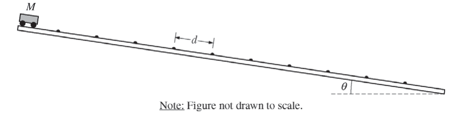
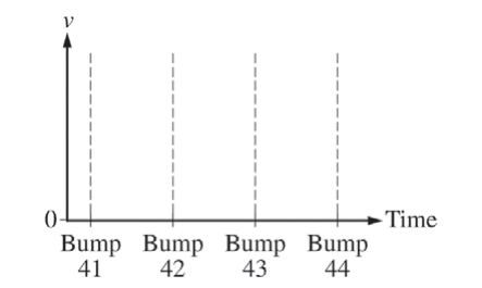
Is the maximum speed of the cart now greater than, less than, or the same as it was with the bumps closer together?
_____ Greater than _____ Less than _____ The same as
Briefly explain your reasoning.
_____ Greater than _____ Less than _____ The same as
Briefly explain your reasoning.
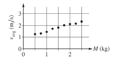
Are these data consistent with the student’s equation?
_____ Yes _____ No
Briefly explain your reasoning.
ii. Another student suggests that whether or not the data above are consistent with the equation, the equation could be incorrect for other reasons. Does the equation make physical sense?
_____ Yes _____ No
Briefly explain your reasoning.
Most-appropriate topic codes (AP Physics 1):
• Topic 2.7 — Kinetic and Static Friction (Parts (b), (c))
• Topic 3.3 — Potential Energy (Parts (b), (c))
• Topic 3.4 — Conservation of Energy (Parts (b), (c))
• Topic 6.5 — Rolling / Translational Motion (Part (a))
▶️ Answer/Explanation
(a)(i) and (ii) — Velocity-time graph
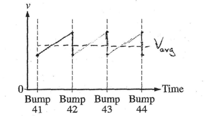
Between bump 41 and bump 44, the cart has already reached its maximum average speed \(v_\text{avg}\). In each interval between two consecutive bumps, the cart accelerates steadily down the ramp (constant net force along the incline), so the velocity increases with a constant positive slope. When the cart hits a bump, it loses some speed almost instantaneously (an abrupt, brief collision), and the velocity resets to the same lower value at the start of each new segment. This produces a repeating sawtooth pattern.
Key features of the correct graph:
• Constant upward slope in each segment between bumps (constant acceleration \(a = g\sin\theta – \) friction-like bump loss).
• Velocity drops abruptly and by the same amount at each bump — the minimum value at the start of each segment is the same for all three intervals.
• The maximum velocity reached just before each bump is the same in each segment (since the motion is now periodic).
• A horizontal dashed line labeled \(v_\text{avg}\) lies between the minimum and maximum velocities, at the time-average of the sawtooth, consistent with equal areas above and below.
The dashed red horizontal line at \(v = v_\text{avg}\) is drawn consistently with the sawtooth, lying between the minimum and maximum values of each cycle.
(b) \(\boxed{\textbf{Greater than}}\)
When the distance \(d\) between bumps is increased, the cart has a longer stretch of ramp over which to accelerate before it encounters the next bump. Since the net force down the ramp is unchanged (same \(\theta\), same \(M\)), the cart spends more time accelerating between bumps, reaching a higher speed just before each bump. Consequently, even after accounting for the energy lost at each bump, the maximum average speed \(v_\text{avg}\) attained between bumps is larger.
Energy perspective: A larger \(d\) means a greater vertical drop \(\Delta h = d\sin\theta\) between successive bumps. More gravitational potential energy \(\Delta U = Mg\,d\sin\theta\) is released between bumps. Even though the same fraction of energy is lost at each bump, the cart gains more kinetic energy per segment, so the maximum speed is greater.
(c) \(\boxed{\textbf{Greater than}}\)
A larger ramp angle \(\theta\) increases the component of gravity directed down the ramp: \[ F_{\parallel} = Mg\sin\theta \] With a larger \(F_{\parallel}\), Newton’s second law gives a greater translational acceleration \(a = g\sin\theta\) along the ramp. The cart therefore gains more speed in each segment between bumps, and the maximum average speed \(v_\text{avg}\) is greater.
Energy perspective: Increasing \(\theta\) increases the vertical height \(\Delta h = d\sin\theta\) between successive bumps (for the same horizontal spacing). More potential energy \(Mg\,d\sin\theta\) is converted to kinetic energy between each pair of bumps, so the cart reaches a higher maximum speed.
(d)(i) \(\boxed{\textbf{No}}\)
The proposed equation is \[ v_\text{avg} = C\frac{Mg\sin\theta}{d} \] which predicts that \(v_\text{avg}\) is directly proportional to \(M\). This means the graph of \(v_\text{avg}\) vs.\ \(M\) should be a straight line passing through the origin (zero \(y\)-intercept) with slope \(Cg\sin\theta/d\).
However, the graph shows:
• The data do not pass through the origin — there is a nonzero \(y\)-intercept, indicating \(v_\text{avg}\) is not proportional to \(M\).
• Doubling the mass from \(M = 1.0\) kg to \(M = 2.0\) kg does not double \(v_\text{avg}\), which the equation would require.
Therefore the data are not consistent with the student’s equation.
(d)(ii) \(\boxed{\textbf{No}}\)
The equation is physically implausible because the distance \(d\) appears in the denominator: \[ v_\text{avg} = C\frac{Mg\sin\theta}{d} \] This predicts that a larger bump spacing \(d\) gives a smaller maximum average speed \(v_\text{avg}\). But from part (b), we reasoned (correctly) that increasing \(d\) gives the cart more distance and time to accelerate, which should increase \(v_\text{avg}\). The equation contradicts this physically motivated conclusion, so the dependence on \(d\) is incorrect and the equation does not make physical sense.
Note: A plausible equation would have \(d\) in the numerator, e.g., \(v_\text{avg} \propto \sqrt{g\,d\sin\theta}\), which is consistent with kinematics: \(v^2 = 2a\,d = 2g\sin\theta\,d\). Such an expression correctly predicts that \(v_\text{avg}\) is independent of \(M\) and increases with both \(d\) and \(\sin\theta\).
Question
Ranking:
Brief explanation:
_____ Increase _____ Decrease _____ Remain the same
Briefly explain your reasoning.
_____ Increase _____ Decrease _____ Remain the same
Briefly explain your reasoning.
Most-appropriate topic codes (AP Physics 2):
• Topic 11.3 — Resistance (Parts (a), (b), (c))
• Topic 11.5 — Compound Direct Current Circuits (Parts (a), (b), (c))
• Topic 11.6 — Kirchhoff’s Loop Rule (Parts (b), (c))
• Topic 11.7 — Kirchhoff’s Junction Rule (Parts (b), (c))
▶️ Answer/Explanation
Circuit Analysis (Original Circuit)
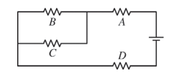
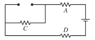
Let each resistor have resistance \(R\) and let the battery EMF be \(\mathcal{E}\). From the circuit diagram, the topology is: resistors \(A\) and \(D\) are in series with the battery, while resistors \(B\) and \(C\) form a parallel combination between \(A\) and \(D\).
The effective resistance of the \(B\)–\(C\) parallel combination is: \( R_{BC} = \dfrac{R \cdot R}{R + R} = \dfrac{R}{2} \)
Total circuit resistance: \( R_\text{total} = R_A + R_{BC} + R_D = R + \dfrac{R}{2} + R = \dfrac{5R}{2} \)
Total (full) current supplied by the battery: \( I = \dfrac{\mathcal{E}}{R_\text{total}} = \dfrac{\mathcal{E}}{\tfrac{5R}{2}} = \dfrac{2\mathcal{E}}{5R} \)
Since \(B\) and \(C\) are identical and in parallel, current splits equally: \( I_B = I_C = \dfrac{I}{2} = \dfrac{\mathcal{E}}{5R} \)
Potential differences across each resistor:
\( \Delta V_A = IR = \dfrac{2\mathcal{E}}{5R} \cdot R = \dfrac{2\mathcal{E}}{5} \), \( \Delta V_D = IR = \dfrac{2\mathcal{E}}{5} \), \( \Delta V_B = I_B R = \dfrac{\mathcal{E}}{5R} \cdot R = \dfrac{\mathcal{E}}{5} \), \( \Delta V_C = \dfrac{\mathcal{E}}{5} \)
Kirchhoff’s Loop Rule check: \( \mathcal{E} = \Delta V_A + \Delta V_B + \Delta V_D = \dfrac{2\mathcal{E}}{5} + \dfrac{\mathcal{E}}{5} + \dfrac{2\mathcal{E}}{5} = \mathcal{E} \checkmark \)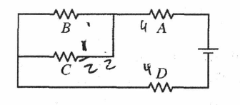
(a)
\( \boxed{(A = D) > (B = C)} \)
• Resistors \(A\) and \(D\) are in series with the battery, so the full current \(I\) flows through each. With identical resistance \(R\), they have equal potential differences: \( \Delta V_A = \Delta V_D = IR \).
• Resistors \(B\) and \(C\) are in parallel. By Kirchhoff’s Junction Rule, the current \(I\) splits equally so each carries \(I/2\), giving \( \Delta V_B = \Delta V_C = (I/2)R \).
• Since \( IR > (I/2)R \), the potential differences across \(A\) and \(D\) are each greater than those across \(B\) and \(C\).
(b) \(\boxed{\textbf{Decrease}}\)
When \(B\) is removed, the parallel \(B\)–\(C\) combination is replaced by \(C\) alone. The new total resistance becomes: \( R_\text{new} = R_A + R_C + R_D = R + R + R = 3R \)
This is larger than the original \( R_\text{total} = \tfrac{5R}{2} = 2.5R \), so the new battery current is: \( I’ = \dfrac{\mathcal{E}}{3R} \approx \dfrac{0.33\,\mathcal{E}}{R} \)
Comparing with the original: \( I = \dfrac{2\mathcal{E}}{5R} \approx \dfrac{0.40\,\mathcal{E}}{R} \)
Since \( I’ < I \), and \(A\) carries the full battery current in both cases, the current through \(A\) decreases. Removing \(B\) replaces a low-resistance parallel combination \((R/2)\) with a single resistor \((R)\), raising the total resistance and thus reducing the total current through \(A\).
(c) \(\boxed{\textbf{Increase}}\)
In the original circuit, current through \(C\) was: \( I_C^\text{original} = \dfrac{I}{2} = \dfrac{\mathcal{E}}{5R} \approx \dfrac{0.20\,\mathcal{E}}{R} \)
After \(B\) is removed, all battery current passes through \(C\): \( I_C^\text{new} = I’ = \dfrac{\mathcal{E}}{3R} \approx \dfrac{0.33\,\mathcal{E}}{R} \)
Since \( \dfrac{0.33\,\mathcal{E}}{R} > \dfrac{0.20\,\mathcal{E}}{R} \), the current through \(C\) increases.
Loop Rule argument: With \(B\) gone, the total resistance of the circuit increased, but the potential difference across the segment containing \(C\) also increased as a fraction of the total EMF. By Ohm’s Law \((\Delta V_C = I_C \cdot R)\), a larger \(\Delta V_C\) across the same \(R\) means a larger \(I_C\).
Junction Rule argument: Previously the current entering the \(B\)–\(C\) node split between \(B\) and \(C\). Now with \(B\) absent, the entire current reaching the node must flow through \(C\). Even though the total battery current decreased, \(C\) now carries all of it rather than half, so \(I_C\) increases.
Question
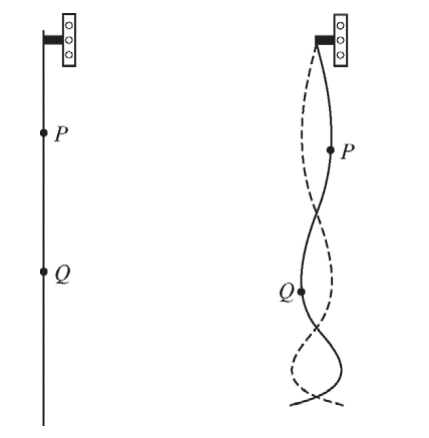
The figure above on the left shows a uniformly thick rope hanging vertically from an oscillator that is turned off. When the oscillator is on and set at a certain frequency, the rope forms the standing wave shown above on the right. \(P\) and \(Q\) are two points on the rope.
Most-appropriate topic codes (AP Physics 2):
• Topic 14.2 — Periodic Waves (Parts (a), (b))
• Topic 14.6 — Wave Interference and Standing Waves (Part (b))
▶️ Answer/Explanation
(a)
Any point on the hanging rope must support the weight of all the rope below it. Consider a small segment of the rope at point \(P\): the upward tension \(T_P\) at that point must balance the downward gravitational force on everything below \(P\). The same argument applies at \(Q\).
Since \(P\) is higher up on the rope than \(Q\), there is more rope — and therefore more mass — hanging below \(P\) than below \(Q\). If the rope has linear mass density \(\mu\) and the lengths of rope below \(P\) and \(Q\) are \(\ell_P\) and \(\ell_Q\) respectively (with \(\ell_P > \ell_Q\)), then:
\( T_P = \mu \, \ell_P \, g \quad > \quad T_Q = \mu \, \ell_Q \, g \)
Therefore the tension at \(P\) is greater than the tension at \(Q\) because the rope at \(P\) must support more weight below it than the rope at \(Q\).
(b) — Paragraph Response
The standing wave pattern on the rope directly supports the student’s hypothesis through the following chain of reasoning. First, notice from the standing wave diagram that the loops — each representing a half-wavelength \(\lambda/2\) — are larger (longer) near the top of the rope, around point \(P\), and become progressively smaller (shorter) toward the bottom, near point \(Q\). This means the local wavelength \(\lambda\) is greater near \(P\) than near \(Q\): \( \lambda_P > \lambda_Q \) Second, since the entire rope is driven by a single oscillator, the frequency \(f\) is the same at every point along the rope. Third, applying the fundamental wave relationship: \( v = \lambda f \) and since \(f\) is constant throughout, a larger wavelength directly implies a larger wave speed. Therefore: \( v_P = \lambda_P f \; > \; v_Q = \lambda_Q f \) meaning the wave travels faster near \(P\) than near \(Q\). Finally, from part (a), the tension is greater near \(P\) (top) than near \(Q\) (bottom), i.e., \(T_P > T_Q\). Putting these two results together: the region of greater tension (\(P\)) also has greater wave speed, and the region of lesser tension (\(Q\)) has lesser wave speed. This is precisely what the student’s hypothesis predicts — that higher tension leads to higher wave speed — and the standing wave pattern on the rope therefore supports it.