ap24-frq-statistics

Question 1

A large exercise center has several thousand members from age $18$ to $55$ years and several thousand members age $56$ and older. The manager of the center is considering offering online fitness classes. The manager is investigating whether members’ opinions of taking online fitness classes differ by age.

The manager selected a random sample of $170$ exercise center members ages $18$ to $55$ years and a second random sample of $230$ exercise center members ages $56$ years and older. Each sampled member was asked whether they would be interested in taking online fitness classes. The manager found that $51$ of the $170$ sampled members ages $18$ to $55$ years and that $79$ of the $230$ sampled members ages $56$ years and older said they would be interested in taking online fitness classes.

At a significance level of $\alpha=0.05$, do the data provide convincing statistical evidence of a difference in the proportion of all exercise center members ages $18$ to $55$ years who would be interested in taking online fitness classes and the proportion of all exercise center members ages $56$ years and older who would be interested in taking online fitness classes? Complete the appropriate inference procedure to justify your response.

Most-appropriate topic codes (AP Statistics):

• Topic $3.12$ — Setting Up a Test for the Difference Between Two Population Proportions (Entire Question)
• Topic $3.13$ — Carrying Out a Test for the Difference Between Two Population Proportions (Entire Question)

▶️ Answer/Explanation

To determine if there’s a significant difference between the two age groups, we will perform a two-sample $z$-test for a difference in population proportions.

First, we need to state our hypotheses.
Let $p_{\text{younger}}$ represent the true proportion of members aged $18$ to $55$ who are interested in taking online fitness classes.
Let $p_{\text{older}}$ represent the true proportion of members aged $56$ and older who are interested in taking online fitness classes.
Null Hypothesis, $H_0: p_{\text{younger}} = p_{\text{older}}$
Alternative Hypothesis, $H_a: p_{\text{younger}} \neq p_{\text{older}}$

Next, we check the conditions:
1. Randomness: Both samples are stated as being randomly selected.
2. Independence ($10\%$ condition): The samples are drawn without replacement, but since $170 \times 10 = 1700$ and $230 \times 10 = 2300$ are both less than the “several thousand” members in each population, the condition is met.
3. Large Counts: The combined proportion is $\hat{p}_c = \dfrac{51 + 79}{170 + 230} = \dfrac{130}{400} = 0.325$.
The expected successes and failures are $170(0.325) = 55.25$, $170(1 – 0.325) = 114.75$, $230(0.325) = 74.75$, and $230(1 – 0.325) = 155.25$. All expected values are at least $10$, so the sampling distribution is approximately normal.

Now, let’s calculate the test statistic and $p$-value.
The sample proportions are $\hat{p}_{\text{younger}} = \dfrac{51}{170} = 0.30$ and $\hat{p}_{\text{older}} = \dfrac{79}{230} \approx 0.3435$.
The test statistic is:
$z = \dfrac{\hat{p}_{\text{younger}} – \hat{p}_{\text{older}}}{\sqrt{\hat{p}_c(1 – \hat{p}_c)\left(\dfrac{1}{n_{\text{younger}}} + \dfrac{1}{n_{\text{older}}}\right)}}$
$z = \dfrac{0.30 – 0.3435}{\sqrt{0.325(1 – 0.325)\left(\dfrac{1}{170} + \dfrac{1}{230}\right)}} \approx -0.91$
For a two-sided test, the $p$-value is $2 \times P(Z < -0.91) \approx 0.362$.

Finally, we state our conclusion:
Because our $p$-value of $0.362$ is much greater than $\alpha = 0.05$, we fail to reject the null hypothesis. We do not have convincing statistical evidence that there is a difference in the true proportions of younger and older members who are interested in taking online fitness classes.

Question 2

A local elementary school decided to sell bottles printed with the school district’s logo as a fund-raiser. The students in the elementary school were asked to sell bottles in three different sizes (small, medium, and large). The relative frequencies of the number of bottles sold for each size by the elementary school were $0.5$ for small bottles, $0.3$ for medium bottles, and $0.2$ for large bottles.

A local middle school also decided to sell bottles as a fund-raiser, using the same three sizes (small, medium, and large). The middle school students sold three times the number of bottles that the elementary school students sold. For the middle school students, the proportion of bottles sold was equal for all three sizes.

(a) Complete the segmented bar graphs representing the relative frequencies of the number of bottles sold for each size by students at each school.

(b) An administrator at the elementary school concluded that the elementary school students sold more small bottles than the middle school students did. Is the elementary school administrator’s conclusion correct? Explain your response.

Two high schools are also selling the bottles and are competing to see which one sold more large bottles.

(c) A mosaic plot for the distribution of the number of bottles sold by each of the high schools is shown here.

i. Which of the two high schools sold a greater proportion of large bottles? Justify your answer.
ii. Which of the two high schools sold a greater number of large bottles? Justify your answer.

Most-appropriate topic codes (AP Statistics):

• Topic $2.1$ — Tabular and Graphical Representations for the Distributions of Two Categorical Variables (Parts $ \mathrm{a} $, $ \mathrm{c} $)
• Topic $2.2$ — Summary Statistics for Two Categorical Variables (Part $ \mathrm{b} $)

▶️ Answer/Explanation

(a)

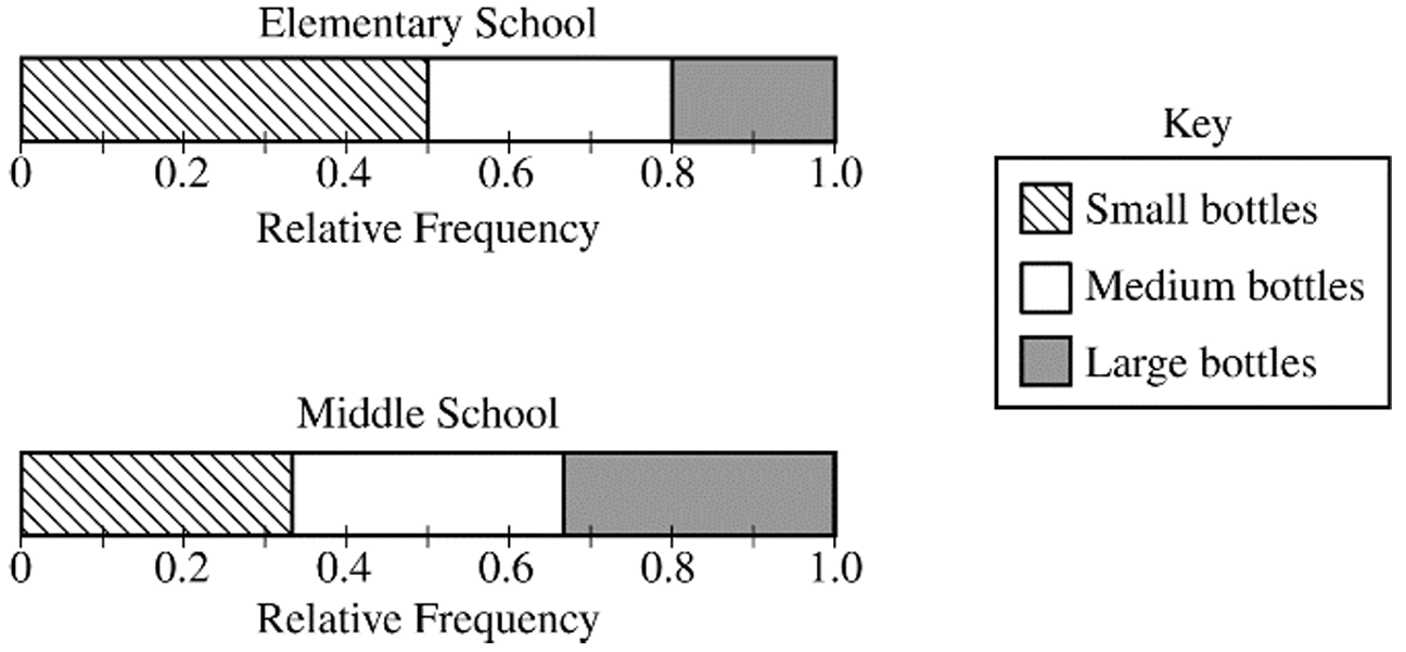
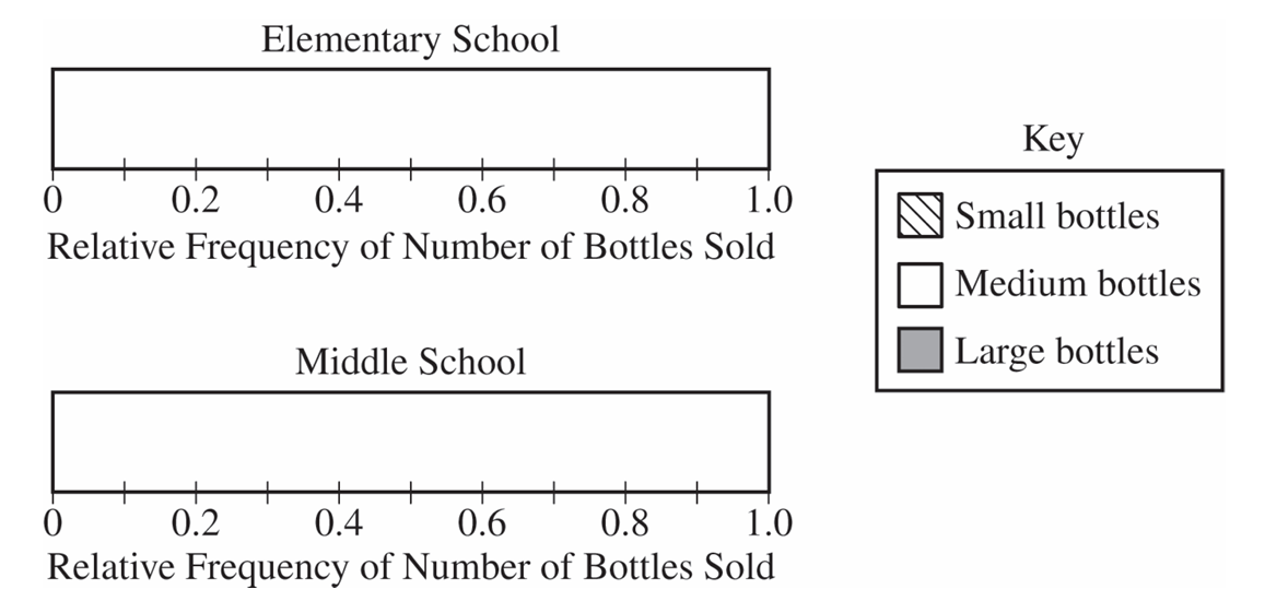
For the Elementary School bar graph, partition the segments at $0.5$ for small bottles, $0.8$ ($0.5 + 0.3$) for medium bottles, and $1.0$ for large bottles.
For the Middle School bar graph, since the proportions are equal, partition the bar into three equal areas at approximately $0.33$ and $0.67$.

(b)
No, the elementary school administrator’s conclusion is incorrect.
Let $x$ represent the total number of bottles sold by the elementary school.
This means the elementary school sold $0.5x$ small bottles.
The middle school sold three times as many total bottles, which is $3x$.
Since the proportion is equal across the three sizes, the middle school sold $\frac{1}{3}(3x) = x$ small bottles.
Because $x > 0.5x$, the middle school actually sold more small bottles than the elementary school.

(c)(i)
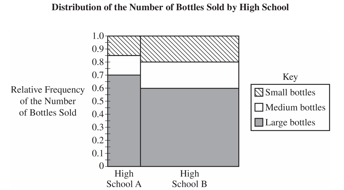
High School A sold a greater proportion of large bottles.
Looking at the y-axis of the mosaic plot, High School A’s proportion for large bottles is $0.7$, which is greater than High School B’s proportion of $0.6$.

(c)(ii)
High School B sold a greater number of large bottles.
In a mosaic plot, the total number of items is represented by the area of the segments.
Even though High School A had a larger proportion, the overall area of the rectangle representing large bottles for High School B is visibly larger than the area for High School A.

Question 3

A car maker produces four different models of cars: A, B, C, and D. A group of researchers is investigating which model of car has the longest distance traveled per gallon of gas (mileage). Higher mileage is considered better than lower mileage. The researchers will conduct a study in which they contact several owners of each model of car and ask them to estimate their mileage.

(a) Is this an observational study or an experiment? Justify your answer in context.

Model D has an autopilot feature, in which the car controls its own motion with human supervision. James owns a Model D car and will investigate whether using the autopilot feature results in higher mileage than not using the autopilot. James will drive his car on $70$ different days to and from work, using the same route at the same time each day. James will record the mileage each day.

(b) James will use a completely randomized design to conduct his investigation. Describe an appropriate method James could use to randomly assign the two treatments, driving using the autopilot feature and driving without using the autopilot feature, to $35$ days each.

(c) After the investigation was completed, James verified that the conditions for inference were met and conducted a hypothesis test. He discovered the mean mileage when using the autopilot feature was significantly higher than the mean mileage when not using the autopilot feature. James is a member of a Model D club with thousands of members who all drive Model D cars. He will give a presentation at a Model D club members’ meeting later this year and would like to state that the results of his hypothesis test apply to all Model D cars in his club. Another member of the club who is a statistician tells James his findings do not apply to all Model D cars in the club. What change would James need to make to his original study to be able to generalize to all Model D cars in the club?

Most-appropriate topic codes (AP Statistics):

• Topic $1.10$ — The Investigative Question Revisited and Data Collection (Parts $ \mathrm{a} $, $ \mathrm{c} $)
• Topic $1.13$ — Experimental Design (Part $ \mathrm{b} $)

▶️ Answer/Explanation

(a)
This is an observational study.
The researchers are simply gathering data by asking car owners to estimate their mileage, without actively imposing any treatments or randomly assigning participants to drive specific car models.

(b)
First, number the $70$ days from $1$ to $70$.
Write the numbers $1$ through $70$ on identical slips of paper, place them into a hat, and mix them thoroughly.
Draw $35$ slips of paper one by one without replacement.
The $35$ days corresponding to the drawn numbers will be assigned the treatment of driving with the autopilot feature, and the remaining $35$ days will be assigned to drive without the autopilot feature.

(c)
In order to generalize his findings to all Model D cars in his club, James cannot solely rely on an experiment conducted using only his own vehicle.
He would need to select a random sample of Model D cars (and their respective drivers) from the club’s membership to participate in his study.

Question 4

In an online game, players move through a virtual world collecting geodes, a type of hollow rock. When broken open, these geodes contain crystals of different colors that are useful in the game. A red crystal is the most useful crystal in the game. The color of the crystal in each geode is independent and the probability that a geode contains a red crystal is $0.08$.

(a) Sarah, a player, will collect and open geodes until a red crystal is found.

i. Calculate the mean of the distribution of the number of geodes Sarah will open until a red crystal is found. Show your work.
ii. Calculate the standard deviation of the distribution of the number of geodes Sarah will open until a red crystal is found. Show your work.

(b) Another player, Conrad, decides to play the game and will stop opening geodes after finding a red crystal or when $4$ geodes have been opened, whichever comes first. Let $Y =$ the number of geodes Conrad will open. The table shows the partially completed probability distribution for the random variable $Y$.

i. Calculate $P(Y=3)$. Show your work.
ii. Calculate $P(Y=4)$. Show your work.

(c) Consider the table and your results from part (b).

i. Calculate the mean of the distribution of the number of geodes Conrad will open. Show your work.
ii. Interpret the mean of the distribution of the number of geodes Conrad will open, which was calculated in part (c-i).

Most-appropriate topic codes (AP Statistics):

• Topic $2.8$ — Introduction to Random Variables and Probability Distributions (Part $ \mathrm{b} $)
• Topic $2.9$ — Parameters of Random Variables (Parts $ \mathrm{a} $, $ \mathrm{c} $)

▶️ Answer/Explanation

(a)
i. Since Sarah opens geodes until she finds a red crystal, the number of geodes she opens follows a geometric distribution with a probability of success $p = 0.08$.
The mean (expected value) of a geometric distribution is $\mu = \dfrac{1}{p}$.
$\mu = \dfrac{1}{0.08} = 12.5$ geodes.
ii. The standard deviation of a geometric distribution is given by $\sigma = \dfrac{\sqrt{1-p}}{p}$.
$\sigma = \dfrac{\sqrt{1-0.08}}{0.08} = \dfrac{\sqrt{0.92}}{0.08} \approx 11.99$ geodes.

(b)
i. The probability that Conrad opens exactly $3$ geodes is the probability of finding non-red crystals in the first two attempts and a red crystal on the third attempt.
$P(Y=3) = (1 – 0.08)^2(0.08) = (0.92)^2(0.08) \approx 0.067712$.
ii. The probability that Conrad opens $4$ geodes is the probability that he does not stop in the first $3$ geodes. He will open 4 geodes whether the 4th is red or not.
$P(Y=4) = 1 – P(Y \le 3)$
$P(Y=4) = 1 – (0.08 + 0.0736 + 0.067712) \approx 0.778688$.

(c)
i. The mean of the discrete probability distribution for $Y$ is the expected value, calculated by summing the products of each outcome and its respective probability.
$\mu_Y = E(Y) = 1(0.08) + 2(0.0736) + 3(0.067712) + 4(0.778688)$
$\mu_Y \approx 0.08 + 0.1472 + 0.203136 + 3.114752 \approx 3.545$ geodes.
ii. The mean of $3.545$ represents the average number of geodes Conrad would open per game if he were to play this game many, many times under the exact same stopping rules.

Question 5

Baseball cards are trading cards that feature data on a player’s performance in baseball games. Michelle is at a national baseball card collector’s convention with approximately $20,000$ attendees. She notices that some collectors have both regular cards, which are easily obtained, and rare cards, which are harder to obtain. Michelle believes that there is a relationship between the number of months a collector has been collecting baseball cards and whether the majority of the cards (cards appearing more often) in their collection are regular or rare. She obtains information from a random sample of $500$ baseball card collectors at the convention and records how many full months they have been collecting baseball cards and whether the majority of the cards in their card collection are regular or rare. Her results are displayed in a two-way table.

Majority Type of Baseball Cards and Months of Collecting Baseball Cards

(a) If one collector from the sample is selected at random, what is the probability that the collector has been collecting baseball cards for $11$ or more months and has a majority of regular baseball cards? Show your work.

(b) Given that a randomly selected collector from the sample has been collecting baseball cards for fewer than $6$ months, what is the probability the collector has a majority of regular baseball cards? Show your work.

(c) Michelle believes there is a relationship between the number of months spent collecting baseball cards and which type of card is the majority in the collection (regular or rare).

i. Name the hypothesis test Michelle should use to investigate her belief. Do not perform the hypothesis test.
ii. State the appropriate null and alternative hypotheses for the hypothesis test you identified in (c-i). Do not perform the hypothesis test.

(d) After completing the hypothesis test described in part (c), Michelle obtains a $p$-value of $0.0075$. Assuming the conditions for inference are met, what conclusion should Michelle make about her belief? Justify your response.

Most-appropriate topic codes (AP Statistics):

• Topic $2.2$ — Summary Statistics for Two Categorical Variables (Parts $ \mathrm{a} $, $ \mathrm{b} $)
• Topic $3.14$ — Setting Up a Chi-Square Test for Homogeneity or Independence (Part $ \mathrm{c} $)
• Topic $3.15$ — Carrying Out a Chi-Square Test for Homogeneity or Independence (Part $ \mathrm{d} $)

▶️ Answer/Explanation

(a)
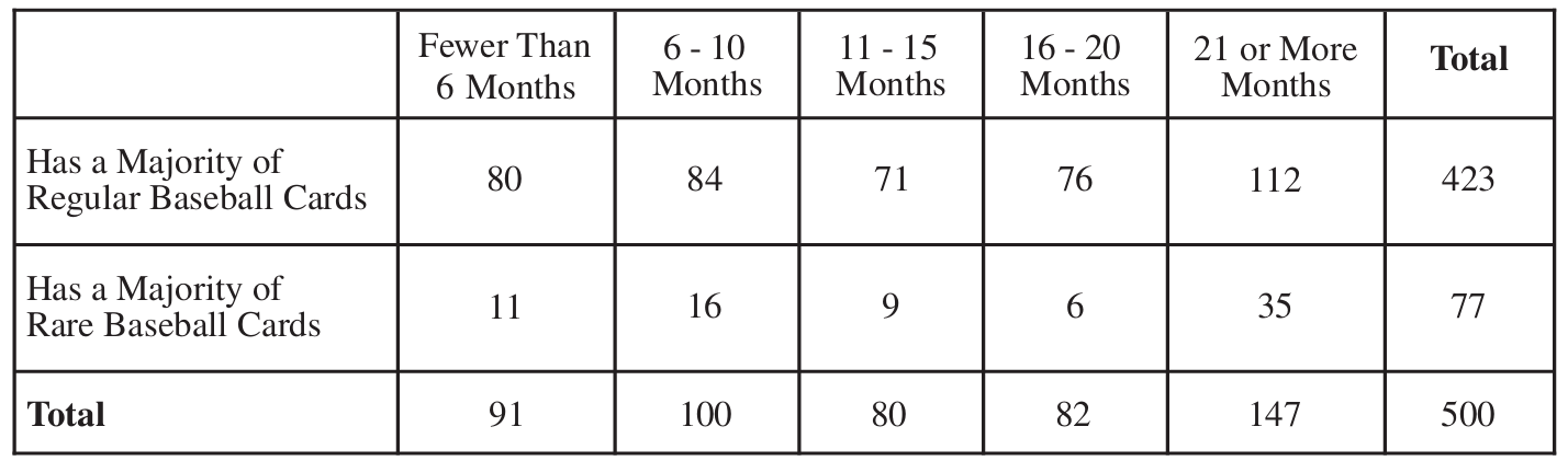
To find this probability, we sum the number of collectors who have a majority of regular cards AND have been collecting for $11$ or more months (which covers the $11-15$, $16-20$, and $21+$ columns).
Number of collectors $= 71 + 76 + 112 = 259$.
$P(\ge 11\text{ months and majority regular}) = \dfrac{259}{500} = 0.518$.

(b)
This is a conditional probability. We restrict our focus entirely to the column representing collectors with fewer than $6$ months of collecting, which gives us a new total of $91$ collectors.
Out of those $91$ collectors, $80$ have a majority of regular baseball cards.
$P(\text{majority regular} \mid < 6\text{ months}) = \dfrac{80}{91} \approx 0.879$.

(c)
i. Because Michelle took a single random sample and is comparing two categorical variables from that single sample, she should use a chi-square test for independence.
ii. Null Hypothesis ($H_0$): There is no association between the number of months spent collecting baseball cards and majority card status for all baseball card collectors at the convention.
Alternative Hypothesis ($H_a$): There is an association between the number of months spent collecting baseball cards and majority card status for all baseball card collectors at the convention.

(d)
Because the $p$-value of $0.0075$ is smaller than any reasonable significance level (such as $\alpha = 0.05$), Michelle should reject the null hypothesis.
The data provide convincing statistical evidence that there is a relationship between the number of months spent collecting baseball cards and which type of card is the majority in the collection for all baseball card collectors at the convention.

Question 6

A company sells a certain type of whistle. The price of the whistle varies from store to store. Julio, a statistician at the company, wants to estimate the mean price, in dollars ($\$\delta$), of this type of whistle at all stores that sell the whistle.

(a)
i. Identify the appropriate inference procedure for Julio to use.
ii. Describe the parameter for the inference procedure you identified in part (a-i) in context.

Julio called the managers of $20$ randomly selected stores that sell the whistle and recorded the price of the whistle at each store. Following is a dotplot of Julio’s data.

The summary statistics for Julio’s data are shown in the following table.

Summary Statistics for Julio’s Data

(b) Julio wants to examine some characteristics of the distribution of the sample of whistle prices.

i. Describe the shape of the distribution of the sample of whistle prices. Justify your response using appropriate values from the summary statistics table.
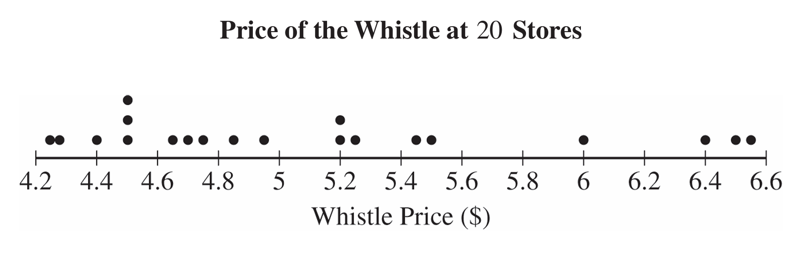
ii. Using the $1.5 \times \text{IQR}$ rule, determine whether there are any outliers in the sample of whistle prices. Justify your response.

It can often be difficult to determine whether the distribution of sample data is skewed by looking at a graph of the data and the summary statistics, particularly when the sample size is small. Thus, statisticians sometimes measure how skewed a data set is. One such measure is Pearson’s coefficient of skewness, which is calculated using the following formula.

$\text{Pearson’s Coefficient of Skewness} = \dfrac{3(\bar{x}-m)}{s}$

In the formula, $\bar{x}$ is the sample mean, $m$ is the sample median, and $s$ is the sample standard deviation.

(c)
i. Calculate Pearson’s coefficient of skewness for Julio’s sample of $20$ whistle prices. Show your work.

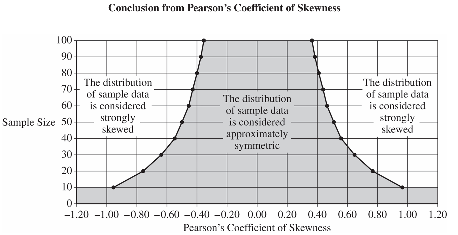The following graph shows conclusions that can be made about the shape of the distribution of sample data based on Pearson’s coefficient of skewness and sample size.

ii. Indicate the value of the Pearson’s coefficient of skewness you calculated in part (c-i) for the appropriate sample size by marking it with an “X” on the preceding graph.

(d) Consider your work in part (c).

i. What should you conclude about the shape of the distribution of the sample of whistle prices? Justify your response.

Julio’s inference procedure in part (a-i) needs one of the following requirements to be satisfied to verify the normality condition.
• The sample size is greater than or equal to $30$.
• If the sample size is less than $30$, the distribution of the sample data is not strongly skewed and does not have outliers.

ii. Using your response to (d-i) and the preceding requirements, is the normality condition satisfied for Julio’s data? Explain your response.

Most-appropriate topic codes (AP Statistics):

• Topic $1.7$ — Summary Statistics for One Quantitative Variable (Parts $ \mathrm{b} $, $ \mathrm{c} $)
• Topic $1.8$ — Graphical Representations of Summary Statistics for One Quantitative Variable (Parts $ \mathrm{b} $, $ \mathrm{c} $)
• Topic $4.2$ — Constructing a Confidence Interval for a Population Mean or Population Mean Difference (Parts $ \mathrm{a} $, $ \mathrm{d} $)

▶️ Answer/Explanation

(a)
i. Julio should use a one-sample $t$-interval for a population mean.
ii. The parameter of interest is $\mu$, the true mean price (in dollars) of this type of whistle at all stores that sell it.

(b)
i. The distribution of the sample of whistle prices is skewed to the right. This is because the mean ($5.12$) is greater than the median ($4.885$).
ii. $\text{IQR} = Q_3 – Q_1 = 5.475 – 4.51 = 0.965$.
Lower boundary: $Q_1 – 1.5(\text{IQR}) = 4.51 – 1.5(0.965) = 3.0625$.
Upper boundary: $Q_3 + 1.5(\text{IQR}) = 5.475 + 1.5(0.965) = 6.9225$.
Since the minimum value ($4.25$) is greater than $3.0625$ and the maximum value ($6.58$) is less than $6.9225$, there are no outliers in the sample.

(c)
i. $\text{Pearson’s Coefficient} = \dfrac{3(5.12 – 4.885)}{0.743} \approx 0.949$.
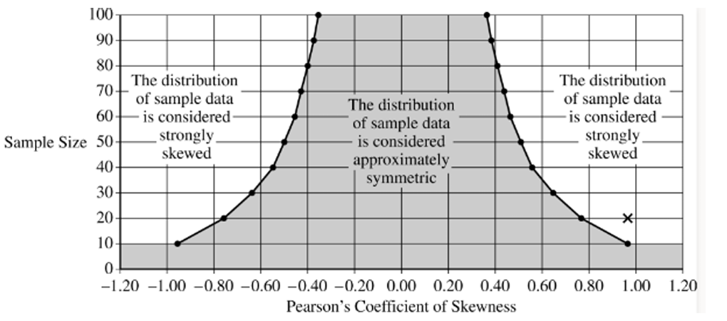
ii. On the graph, you would plot an “X” at a sample size of $y = 20$ and a skewness coefficient of $x \approx 0.949$.

(d)
i. We can conclude that the distribution of the sample of whistle prices is strongly skewed. This is justified because the calculated coefficient of $0.949$ for a sample size of $20$ falls in the “strongly skewed” region of the provided graph.
ii. No, the normality condition is not satisfied. The sample size ($n = 20$) is less than $30$, and although there are no outliers, the sample data is strongly skewed, failing the second condition.

Question 1

Question 2

Question 3

Question 4

Question 5

Question 6

Resources

Members

Company