Home / AP_Statistics_2019_FRQ

Question 1

The sizes, in square feet, of the \(20\) rooms in a student residence hall at a certain university are summarized in the following histogram.
(a) Based on the histogram, write a few sentences describing the distribution of room size in the residence hall.
(b) Summary statistics for the sizes are given in the following table.
MeanStandard DeviationMinQ1MedianQ3Max
\(231.4\)\(68.12\)\(134\)\(174\)\(253.5\)\(292\)\(315\)
Determine whether there are potential outliers in the data. Then use the following grid to sketch a boxplot of room size.
(c) What characteristic of the shape of the distribution of room size is apparent from the histogram but not from the boxplot?

Most-appropriate topic codes (CED):

TOPIC 1.6: Describing the Distribution of a Quantitative Variable
TOPIC 1.7: Summary Statistics for a Quantitative Variable
TOPIC 1.8: Graphical Representations of Summary Statistics

▶️ Answer/Explanation
Detailed solution

(a)
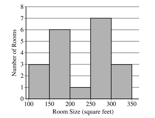
The distribution of room sizes is bimodal, with two distinct clusters of data. One cluster is between \(150\) and \(200\) square feet, and the other is between \(250\) and \(300\) square feet. The distribution is roughly symmetric with a center between \(200\) and \(250\) square feet. The range of the data is approximately \(350 – 100 = 250\) square feet.

(b)
First, determine potential outliers using the \(1.5 \times IQR\) rule.
– \(IQR = Q_3 – Q_1 = 292 – 174 = 118\).
– Lower Fence: \(Q_1 – 1.5(IQR) = 174 – 1.5(118) = 174 – 177 = -3\).
– Upper Fence: \(Q_3 + 1.5(IQR) = 292 + 1.5(118) = 292 + 177 = 469\).
Since the minimum value (\(134\)) is greater than the lower fence and the maximum value (\(315\)) is less than the upper fence, there are no potential outliers.

The boxplot is sketched below:
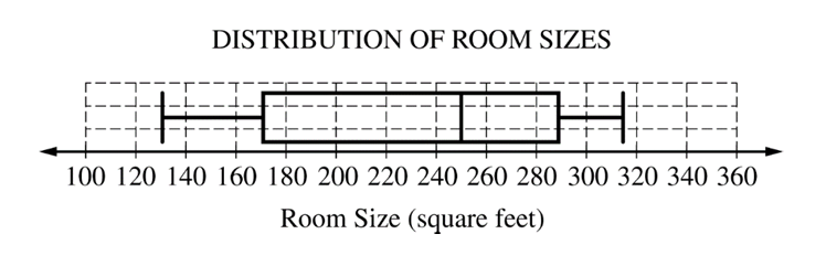
(c)
The most apparent characteristic visible in the histogram but not the boxplot is the **bimodal shape** of the distribution. The histogram clearly shows two distinct peaks, while the boxplot only shows a symmetric distribution with a wide interquartile range, hiding the two separate clusters of data.

Question 2

Researchers are investigating the effectiveness of using a fungus to control the spread of an insect that destroys trees. The researchers will create four different concentrations of fungus mixtures: \(0\) milliliters per liter (ml/L), \(1.25\) ml/L, \(2.5\) ml/L, and \(3.75\) ml/L. An equal number of the insects will be placed into \(20\) individual containers. The group of insects in each container will be sprayed with one of the four mixtures, and the researchers will record the number of insects that are still alive in each container one week after spraying.
(a) Identify the treatments, experimental units, and response variable of the experiment.
  • Treatments:
  • Experimental units:
  • Response variable:
(b) Does the experiment have a control group? Explain your answer.
(c) Describe how the treatments can be randomly assigned to the experimental units so that each treatment has the same number of units.

Most-appropriate topic codes (CED):

TOPIC 3.5: Introduction to Experimental Design — parts (a), (b), (c)
▶️ Answer/Explanation
Detailed solution

(a)

  • Treatments: The four different concentrations of the fungus mixture: \(0\) ml/L, \(1.25\) ml/L, \(2.5\) ml/L, and \(3.75\) ml/L.
  • Experimental units: The \(20\) individual containers, each containing an equal number of insects.
  • Response variable: The number of insects that are still alive in each container one week after spraying.

(b)
Yes, the experiment has a control group. The group of containers that will be sprayed with the mixture containing \(0\) ml/L of fungus serves as the control group. This is because this group is treated in the same way as all other groups but does not receive the active ingredient (the fungus). This provides a baseline to which the effects of the other fungus concentrations can be compared.

(c)
To randomly assign the treatments, we can use the following process:

  1. Label each of the \(20\) containers with a unique number from \(1\) to \(20\).
  2. Create \(20\) identical slips of paper. On five slips, write “\(0\) ml/L”. On another five slips, write “\(1.25\) ml/L”. On another five, write “\(2.5\) ml/L”, and on the final five, write “\(3.75\) ml/L”.
  3. Place all \(20\) slips of paper into a hat or a box and mix them thoroughly.
  4. For each container (from \(1\) to \(20\)), draw one slip of paper from the hat without replacement. Assign the treatment written on the slip to that container.

This process ensures that each treatment is assigned to exactly five containers, and the assignment is completely random.

Question 3

A medical researcher surveyed a large group of men and women about whether they take medicine as prescribed. The responses were categorized as never, sometimes, or always. The relative frequency of each category is shown in the table.
 NeverSometimesAlwaysTotal
Men\(0.0564\)\(0.2016\)\(0.2120\)\(0.4700\)
Women\(0.0636\)\(0.1384\)\(0.3280\)\(0.5300\)
Total\(0.1200\)\(0.3400\)\(0.5400\)\(1.0000\)
(a) One person from those surveyed will be selected at random.
(i) What is the probability that the person selected will be someone whose response is never and who is a woman?
(ii) What is the probability that the person selected will be someone whose response is never or who is a woman?
(iii) What is the probability that the person selected will be someone whose response is never given that the person is a woman?
(b) For the people surveyed, are the events of being a person whose response is never and being a woman independent? Justify your answer.
(c) Assume that, in a large population, the probability that a person will always take medicine as prescribed is \(0.54\). If \(5\) people are selected at random from the population, what is the probability that at least \(4\) of the people selected will always take medicine as prescribed? Support your answer.

Most-appropriate topic codes (CED):

TOPIC 4.3: Introduction to Probability — part (a)
TOPIC 4.6: Independent Events — part (b)
TOPIC 4.10: Introduction to the Binomial Distribution — part (c)
▶️ Answer/Explanation
Detailed solution

(a)
(i) The probability that the person selected is a woman who responds “never” is the joint relative frequency found in the intersection of the “Women” row and the “Never” column.
\(P(\text{Never} \cap \text{Woman}) = 0.0636\).

\(\boxed{0.0636}\)

(ii) The probability that the person selected is a woman or responds “never” is found using the general addition rule: \(P(A \cup B) = P(A) + P(B) – P(A \cap B)\).
From the table, \(P(\text{Never}) = 0.1200\) and \(P(\text{Woman}) = 0.5300\). We found \(P(\text{Never} \cap \text{Woman})\) in part (i). \[ P(\text{Never} \cup \text{Woman}) = 0.1200 + 0.5300 – 0.0636 = 0.5864 \]

\(\boxed{0.5864}\)

(iii) The probability that the person responds “never” given that the person is a woman is a conditional probability. \[ P(\text{Never} | \text{Woman}) = \frac{P(\text{Never} \cap \text{Woman})}{P(\text{Woman})} \] \[ P(\text{Never} | \text{Woman}) = \frac{0.0636}{0.5300} = 0.12 \]

\(\boxed{0.12}\)

(b)
Yes, the events are independent. Two events A and B are independent if \(P(A|B) = P(A)\).
From part (a-iii), we found \(P(\text{Never} | \text{Woman}) = 0.12\).
From the “Total” row of the table, the marginal probability \(P(\text{Never}) = 0.1200\).
Since \(P(\text{Never} | \text{Woman}) = P(\text{Never})\) (\(0.12 = 0.12\)), the event of being a person whose response is “never” is independent of the event of being a woman.

(c)
Let \(X\) be the random variable for the number of people who will always take their medicine as prescribed. This scenario follows a binomial distribution because there is a fixed number of trials (\(n=5\)), each trial is independent, there are two outcomes (always takes medicine or not), and the probability of success is constant (\(p=0.54\)).

So, \(X \sim \text{Binomial}(n=5, p=0.54)\). We want to find the probability that at least \(4\) people always take their medicine, which is \(P(X \ge 4) = P(X=4) + P(X=5)\).

We use the binomial probability formula: \(P(X=k) = \binom{n}{k}p^k(1-p)^{n-k}\).

For \(X=4\): \[ P(X=4) = \binom{5}{4}(0.54)^4(1-0.54)^{5-4} = 5(0.54)^4(0.46)^1 \approx 0.19557 \] For \(X=5\): \[ P(X=5) = \binom{5}{5}(0.54)^5(1-0.54)^{5-5} = 1(0.54)^5(0.46)^0 \approx 0.04592 \] Now we add the probabilities: \[ P(X \ge 4) = 0.19557 + 0.04592 = 0.24149 \]

\(\boxed{0.2415}\)

Question 4

Tumbleweed, commonly found in the western United States, is the dried structure of certain plants that are blown by the wind. Kochia, a type of plant that turns into tumbleweed at the end of the summer, is a problem for farmers because it takes nutrients away from soil that would otherwise go to more beneficial plants. Scientists are concerned that kochia plants are becoming resistant to the most commonly used herbicide, glyphosate. In \(2014\), \(19.7\) percent of \(61\) randomly selected kochia plants were resistant to glyphosate. In \(2017\), \(38.5\) percent of \(52\) randomly selected kochia plants were resistant to glyphosate. Do the data provide convincing statistical evidence, at the level of \(\alpha=0.05\), that there has been an increase in the proportion of all kochia plants that are resistant to glyphosate?

Most-appropriate topic codes (CED):

TOPIC 6.10: Setting Up a Test for the Difference of Two Population Proportions
TOPIC 6.11: Carrying Out a Test for the Difference of Two Population Proportions
▶️ Answer/Explanation
Detailed solution

State:
We will perform a two-sample z-test for a difference in proportions at a significance level of \(\alpha=0.05\). Let \(p_{14}\) be the true proportion of all kochia plants resistant to glyphosate in \(2014\), and let \(p_{17}\) be the true proportion in \(2017\).

The hypotheses are:
\(H_0: p_{17} – p_{14} = 0\)
\(H_a: p_{17} – p_{14} > 0\)


Plan:
We must check the conditions for inference.
1. Random: The data come from two independent random samples of kochia plants.
2. Independence (10% condition): It is reasonable to assume the population of all kochia plants is much larger than \(10 \times 61 = 610\) in \(2014\) and \(10 \times 52 = 520\) in \(2017\).
3. Normality (Large Counts):
– \(\hat{p}_{14} = 0.197\), \(\hat{p}_{17} = 0.385\).
– Pooled proportion: \(\hat{p}_c = \frac{(61)(0.197) + (52)(0.385)}{61+52} = \frac{12.017 + 20.02}{113} \approx 0.2835\).
– Expected counts: \(n_{14}\hat{p}_c = 61(0.2835) \approx 17.29\), \(n_{14}(1-\hat{p}_c) \approx 43.71\), \(n_{17}\hat{p}_c = 52(0.2835) \approx 14.74\), \(n_{17}(1-\hat{p}_c) \approx 37.26\). All expected counts are \(\ge 10\).
All conditions are met.


Do:
Calculate the z-test statistic:
\(z = \frac{(\hat{p}_{17} – \hat{p}_{14}) – 0}{\sqrt{\hat{p}_c(1-\hat{p}_c)(\frac{1}{n_{17}} + \frac{1}{n_{14}})}}\)
\(z = \frac{0.385 – 0.197}{\sqrt{(0.2835)(0.7165)(\frac{1}{52} + \frac{1}{61})}} \approx \frac{0.188}{0.0851} \approx 2.21\)

Find the p-value for the one-sided test:
p-value = \(P(Z > 2.21) \approx 0.0135\)


Conclude:
Since the p-value (\(0.0135\)) is less than the significance level (\(\alpha = 0.05\)), we reject the null hypothesis.

There is convincing statistical evidence to conclude that there has been an increase in the proportion of all kochia plants in the western United States that are resistant to glyphosate between \(2014\) and \(2017\).

Question 5

A company that manufactures smartphones developed a new battery that has a longer life span than that of a traditional battery. From the date of purchase of a smartphone, the distribution of the life span of the new battery is approximately normal with mean \(30\) months and standard deviation \(8\) months. For the price of \(\$50\), the company offers a two-year warranty on the new battery for customers who purchase a smartphone. The warranty guarantees that the smartphone will be replaced at no cost to the customer if the battery no longer works within \(24\) months from the date of purchase.
(a) In how many months from the date of purchase is it expected that \(25\) percent of the batteries will no longer work? Justify your answer.
(b) Suppose one customer who purchases the warranty is selected at random. What is the probability that the customer selected will require a replacement within \(24\) months from the date of purchase because the battery no longer works?
(c) The company has a gain of \(\$50\) for each customer who purchases a warranty but does not require a replacement. The company has a loss (negative gain) of \(\$150\) for each customer who purchases a warranty and does require a replacement. What is the expected value of the gain for the company for each warranty purchased?

Most-appropriate topic codes (CED):

TOPIC 1.10: The Normal Distribution — parts (a), (b)
TOPIC 4.8: Mean and Standard Deviation of Random Variables — part (c)
▶️ Answer/Explanation
Detailed solution

(a)
We need to find the 25th percentile of the normal distribution for battery life span, which has a mean \(\mu = 30\) months and a standard deviation \(\sigma = 8\) months. First, we find the z-score corresponding to the 25th percentile of the standard normal distribution. This value is approximately \(z \approx -0.674\).

Next, we convert this z-score back to the original scale (in months) using the formula \(X = \mu + z\sigma\). \[ X = 30 + (-0.674)(8) \] \[ X = 30 – 5.392 = 24.608 \] So, it is expected that \(25\) percent of the batteries will no longer work within approximately \(24.6\) months.

\(\boxed{24.6 \text{ months}}\)

(b)
We need to find the probability that a battery’s life span is less than \(24\) months, i.e., \(P(X < 24)\). We first calculate the z-score for \(X = 24\). \[ z = \frac{X – \mu}{\sigma} = \frac{24 – 30}{8} = \frac{-6}{8} = -0.75 \] Now, we find the probability \(P(Z < -0.75)\) using a standard normal table or calculator. \[ P(X < 24) = P(Z < -0.75) \approx 0.2266 \] The probability that a customer will require a replacement within \(24\) months is approximately \(0.2266\).

\(\boxed{0.2266}\)

(c)
The expected value of the gain is calculated by summing the products of each outcome and its probability. Let \(G\) be the random variable for the company’s gain.

There are two outcomes:

  1. Replacement required: The battery fails within \(24\) months. The gain is \(-\$150\). The probability of this, from part (b), is \(P(X \le 24) = 0.2266\).
  2. No replacement required: The battery lasts longer than \(24\) months. The gain is \(\$50\). The probability is \(P(X > 24) = 1 – P(X \le 24) = 1 – 0.2266 = 0.7734\).

The expected value is: \[ E(G) = (-\$150) \times P(X \le 24) + (\$50) \times P(X > 24) \] \[ E(G) = (-\$150)(0.2266) + (\$50)(0.7734) \] \[ E(G) = -\$33.99 + \$38.67 = \$4.68 \] The expected value of the gain for the company for each warranty purchased is \(\$4.68\).

\(\boxed{\$4.68}\)

Question 6

Emma is moving to a large city and is investigating typical monthly rental prices of available one-bedroom apartments. She obtained a random sample of rental prices for \(50\) one-bedroom apartments taken from a Web site where people voluntarily list available apartments.
(a) Describe the population for which it is appropriate for Emma to generalize the results from her sample.
The distribution of the \(50\) rental prices of the available apartments is shown in the following histogram.
(b) Emma wants to estimate the typical rental price of a one-bedroom apartment in the city. Based on the distribution shown, what is a disadvantage of using the mean rather than the median as an estimate of the typical rental price?
(c) Instead of using the sample median as the point estimate for the population median, Emma wants to use an interval estimate. However, computing an interval estimate requires knowing the sampling distribution of the sample median for samples of size \(50\). Emma has one point, her sample median, in that sampling distribution. Using information about rental prices that are available on the Web site, describe how someone could develop a theoretical sampling distribution of the sample median for samples of size \(50\).

Because Emma does not have the resources to develop the theoretical sampling distribution, she estimates the sampling distribution of the sample median using a process called bootstrapping. In the bootstrapping process, a computer program performs the following steps.
• Take a random sample, with replacement, of size \(50\) from the original sample.
• Calculate and record the median of the sample.
• Repeat the process to obtain a total of \(15,000\) medians.

Emma ran the bootstrap process, and the following frequency table is the bootstrap distribution showing her results of generating \(15,000\) medians.

Bootstrap Distribution of Medians
MedianFrequencyMedianFrequencyMedianFrequency
\(2,345\)\(1\)\(2,585\)\(1\)\(2,825\)\(247\)
\(2,390\)\(13\)\(2,587.5\)\(171\)\(2,837.5\)\(7\)
\(2,395\)\(18\)\(2,600\)\(22\)\(2,847.5\)\(1\)
\(2,400\)\(56\)\(2,612.5\)\(1,190\)\(2,872.5\)\(317\)
\(2,445\)\(4\)\(2,625\)\(174\)\(2,885\)\(10\)
\(2,447.5\)\(56\)\(2,672.5\)\(5\)\(2,950\)\(700\)
\(2,450\)\(55\)\(2,675\)\(1,924\)\(2,962.5\)\(93\)
\(2,475\)\(3\)\(2,687.5\)\(1,341\)\(2,972.5\)\(6\)
\(2,495\)\(66\)\(2,700\)\(2,825\)\(2,975\)\(65\)
\(2,497.5\)\(136\)\(2,735\)\(35\)\(2,985\)\(12\)
\(2,500\)\(1,899\)\(2,747.5\)\(619\)\(2,987.5\)\(1\)
\(2,522.5\)\(2\)\(2,750\)\(2\)\(2,995\)\(6\)
\(2,525\)\(945\)\(2,795\)\(278\)\(3,000\)\(2\)
\(2,550\)\(1,673\)\(2,812.5\)\(16\)\(3,062.5\)\(3\)
(d) Use the frequency table to find the following.
(i) Value of the \(5^{th}\) percentile:
(ii) Value of the \(95^{th}\) percentile:
(e) Find the percentage of bootstrap medians in the table that are equal to or between the values found in part (d).
(f) Use your values from parts (d) and (e) to construct and interpret a confidence interval for the median rental price.

Most-appropriate topic codes (CED):

TOPIC 3.2: Introduction to Planning a Study
TOPIC 1.6: Describing the Distribution of a Quantitative Variable
TOPIC 5.1: Introducing Statistics: Why Is My Sample Not Like Yours?
▶️ Answer/Explanation
Detailed solution

(a)
Because the sample was taken from a Web site where people voluntarily list available apartments, the results can be generalized to the population of one-bedroom apartments listed on that particular Web site for that city.

(b)
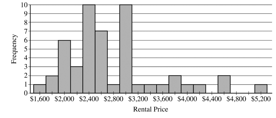
The histogram shows that the distribution of rental prices is skewed to the right. In a right-skewed distribution, the mean is pulled toward the long tail of higher prices and will be greater than the median. This would lead to an overestimation of the typical rental price.

(c)
To create the theoretical sampling distribution, one would have to take every possible unique random sample of size \(50\) from the entire population of apartment listings on the Web site. Then, the median for each of these samples would be calculated. The distribution of all these sample medians would form the theoretical sampling distribution.

(d)
(i) The \(5^{th}\) percentile is at position \(15,000 \times 0.05 = 750\). Summing the frequencies from the start of the table, we find the \(750^{th}\) value falls within the group of medians with a value of \(\$2,500\).
(ii) The \(95^{th}\) percentile is at position \(15,000 \times 0.95 = 14,250\). Summing the frequencies, we find the \(14,250^{th}\) value falls within the group of medians with a value of \(\$2,950\).

(e)
We need to find the percentage of the \(15,000\) medians that are between \(\$2,500\) and \(\$2,950\), inclusive. The number of medians less than \(\$2,500\) is \(1+13+18+56+4+56+55+3+66+136 = 408\). The number of medians greater than \(\$2,950\) is \(93+6+65+12+1+6+2+3 = 188\).
The number of medians at or between these values is \(15,000 – 408 – 188 = 14,404\).
Percentage = \(\frac{14,404}{15,000} \times 100\% \approx 96.03\%\).

(f)
An approximate \(96\%\) confidence interval for the median rental price is \((\$2,500, \$2,950)\).

Interpretation: We are approximately \(96\%\) confident that the true median rental price of all one-bedroom apartments listed on this Web site for this city is between \(\$2,500\) and \(\$2,950\).

Scroll to Top