Systematic and Random Errors in Measurements
All measurements in physics are subject to some form of error the difference between the measured value and the true value of a physical quantity. Understanding and minimizing these errors is essential to improve the accuracy and reliability of experimental results.
Types of Errors in Measurement:
| Error Type | Definition | Cause | Effect on Results | Reduction / Correction |
|---|---|---|---|---|
| Systematic Error | Error that causes all measurements to deviate from the true value by a fixed amount in the same direction (either all too high or all too low). | Faulty equipment, incorrect calibration, zero error, or consistent observer bias. | Affects accuracy — shifts all values by the same amount; cannot be reduced by repetition. | Identify and correct source (e.g., recalibrate instrument, apply correction for zero error). |
| Random Error | Error that causes measurements to fluctuate unpredictably around the true value due to uncontrollable variations. | Environmental changes, human reaction time, or limitations of instrument precision. | Affects precision — leads to scatter of readings; averages may still be close to the true value. | Take multiple readings and calculate the mean; use instruments with finer scale divisions. |
Zero Error (a type of Systematic Error):
- Occurs when an instrument reads a non-zero value even when the measured quantity should be zero.
- Example: A vernier caliper that reads \( \mathrm{+0.02\,mm} \) when fully closed has a +0.02 mm zero error.
- Correction: Subtract or add the zero error value from all readings as appropriate.
Comparison Between Systematic and Random Errors:
| Aspect | Systematic Error | Random Error |
|---|---|---|
| Nature | Consistent deviation in one direction | Unpredictable variations around true value |
| Effect on Accuracy | Decreases accuracy (biases results) | Decreases precision (scatter in data) |
| Detection | Difficult to detect by repetition alone | Detected by irregular fluctuations between readings |
| Reduction Method | Calibration, correction, or elimination of source | Increase number of readings and average |
Example
1. A stopwatch starts \( \mathrm{0.2\,s} \) late every time it is used.
2. A student repeatedly measures the length of a wire and records slightly different values each time. Identify the Error Types
▶️ Answer / Explanation
Case 1: Stopwatch delay = constant shift = Systematic error (zero or calibration error). Correction: Subtract \( \mathrm{0.2\,s} \) from each timing.
Case 2: Small variations between measurements = Random error. Correction: Take multiple readings and average them to reduce effect.
Distinction Between Precision and Accuracy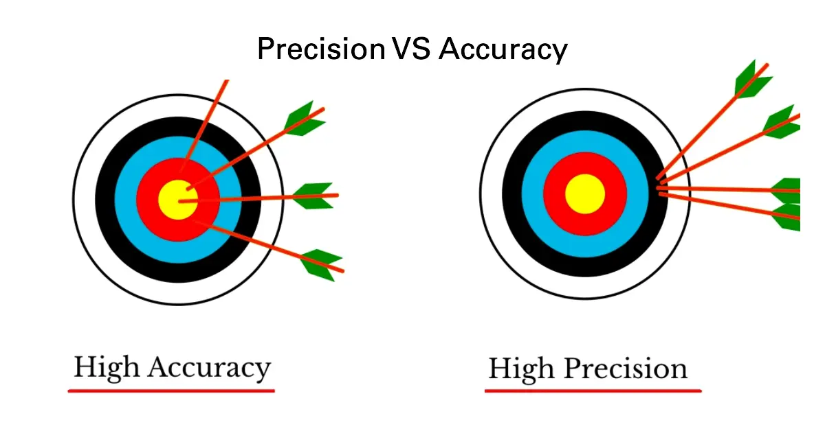
In experimental physics, precision and accuracy describe different aspects of the quality of a measurement. While they are often used together, they do not mean the same thing.
Key Idea:
- Precision is about consistency — how close repeated measurements are to each other.
- Accuracy is about truth — how close a measurement is to the true or accepted value.
Comparison Between Precision and Accuracy:
| Aspect | Precision | Accuracy |
|---|---|---|
| Meaning | How close repeated measurements are to each other. | How close a measurement is to the true or accepted value. |
| Dependence | Affected by random errors. | Affected by systematic errors. |
| Indicator | Small variation or scatter between readings. | Small deviation from the true value. |
| Improved by | Taking repeated readings and averaging results. | Calibrating instruments and correcting systematic errors. |
| Example | Repeated measurements of length are all \( \mathrm{10.02\,cm} \), \( \mathrm{10.03\,cm} \), \( \mathrm{10.02\,cm} \). | Mean measured length \( \mathrm{10.0\,cm} \) is close to the true value \( \mathrm{10.00\,cm} \). |
| Effect on Data Spread | High precision → small spread of readings. | High accuracy → readings centred near the true value. |
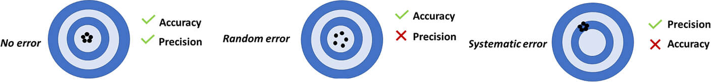
Visual Analogy (Conceptual Explanation):
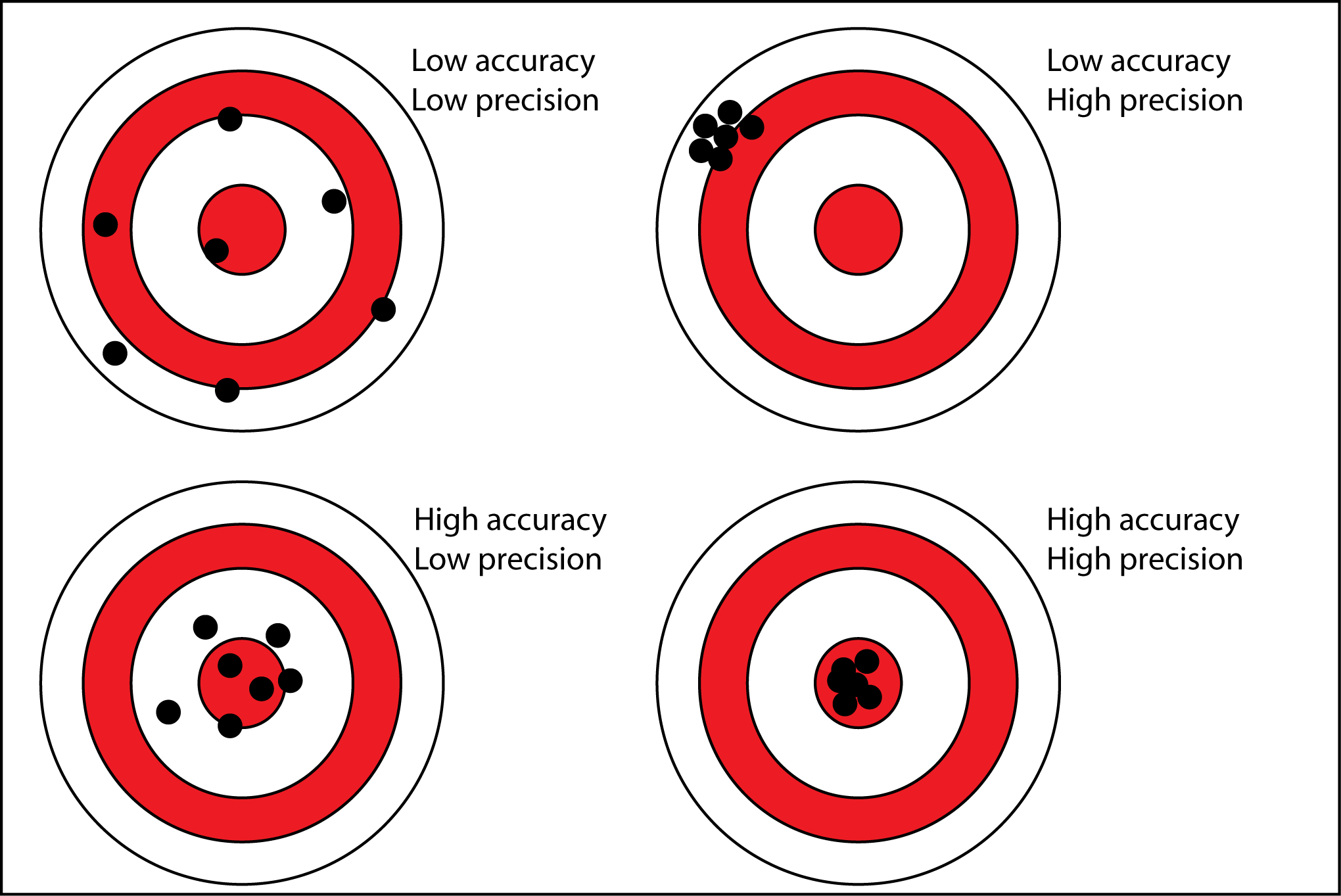
| Condition | Description |
|---|---|
| High Precision, Low Accuracy | All readings are close together but far from the true value (consistent but wrong). |
| Low Precision, High Accuracy | Readings are spread out but the average is close to the true value. |
| High Precision, High Accuracy | All readings are close together and close to the true value (ideal measurement). |
| Low Precision, Low Accuracy | Readings are spread out and far from the true value (poor measurement). |
Example
Understanding Precision vs Accuracy
A student measures the diameter of a wire using a micrometer screw gauge and records:
\( \mathrm{1.23\,mm,\, 1.22\,mm,\, 1.24\,mm,\, 1.23\,mm} \)
The true diameter is \( \mathrm{1.50\,mm} \).
▶️ Answer / Explanation
Step 1: The readings are very close to each other → high precision.
Step 2: However, all are far from the true value → low accuracy.
Conclusion: The instrument may have a systematic error (e.g., zero error). It produces consistent but incorrect readings — precise but not accurate.