Distance, Displacement, Speed, Velocity, and Acceleration
These are the fundamental quantities used to describe motion. They can be classified as scalars or vectors depending on whether direction is involved.
Key Idea:
- Distance and Speed are scalar quantities (only magnitude).
- Displacement, Velocity, and Acceleration are vector quantities (magnitude and direction).
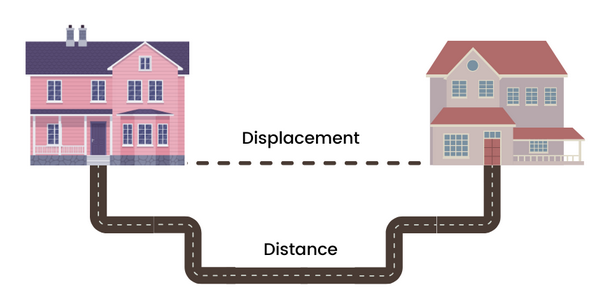
Distance (\( \mathrm{s} \))
- It is the total path length travelled by an object, irrespective of direction.
- Always positive and increases with movement.
- Scalar quantity.
Unit: \( \mathrm{metre\ (m)} \)
Example: A car travels 5 m east and 5 m west — the total distance is \( \mathrm{10\,m.} \)
Displacement (\( \mathrm{\vec{s}} \))
- The shortest straight-line distance between the initial and final positions of an object, in a specific direction.
- Vector quantity — has both magnitude and direction.
Unit: \( \mathrm{metre\ (m)} \)
Example: In the same journey above (5 m east, then 5 m west), the displacement is \( \mathrm{0\,m} \), since the object ends up at its starting point.
Speed (\( \mathrm{v} \))
- Rate of change of distance with respect to time.
- Measures how fast an object moves, without direction.
- Scalar quantity.

Formula:
\( \mathrm{speed = \dfrac{distance}{time}} \)
\( \mathrm{v = \dfrac{s}{t}} \)
Unit: \( \mathrm{m/s} \)
Example: If a cyclist covers \( \mathrm{100\,m} \) in \( \mathrm{20\,s} \), then \( \mathrm{v = 100/20 = 5.0\,m/s.} \)
Velocity (\( \mathrm{\vec{v}} \))
- Rate of change of displacement with respect to time.
- Indicates both speed and direction of motion.
- Vector quantity.

Formula:
\( \mathrm{\vec{v} = \dfrac{\vec{s}}{t}} \)
Average velocity: \( \mathrm{\vec{v}_{avg} = \dfrac{\text{total displacement}}{\text{total time}}} \)
Unit: \( \mathrm{m/s} \)
Instantaneous velocity: Velocity of the body at a particular instant of time.
Acceleration (\( \mathrm{\vec{a}} \))
- Rate of change of velocity with respect to time.
- Measures how quickly the velocity changes in magnitude or direction.
- Vector quantity.

Formula:
\( \mathrm{\vec{a} = \dfrac{\Delta \vec{v}}{\Delta t} = \dfrac{\vec{v} – \vec{u}}{t}} \)
where:
- \( \mathrm{\vec{u}} \): initial velocity
- \( \mathrm{\vec{v}} \): final velocity
- \( \mathrm{t} \): time taken
Unit: \( \mathrm{m/s^2} \)
Types of acceleration:
- Uniform acceleration: Velocity changes at a constant rate (e.g., freely falling body).
- Non-uniform acceleration: Rate of change of velocity is not constant.
Relationship Between the Quantities:
\( \mathrm{speed = \dfrac{distance}{time}} \)
\( \mathrm{velocity = \dfrac{displacement}{time}} \)
\( \mathrm{acceleration = \dfrac{change\ in\ velocity}{time}} \)
Comparison Table:
| Quantity | Definition | Vector / Scalar | SI Unit |
|---|---|---|---|
| Distance | Total path length | Scalar | \( \mathrm{m} \) |
| Displacement | Straight-line distance in a specific direction | Vector | \( \mathrm{m} \) |
| Speed | Rate of change of distance | Scalar | \( \mathrm{m/s} \) |
| Velocity | Rate of change of displacement | Vector | \( \mathrm{m/s} \) |
| Acceleration | Rate of change of velocity | Vector | \( \mathrm{m/s^2} \) |
Example
A car increases its velocity from \( \mathrm{10\,m/s} \) to \( \mathrm{20\,m/s} \) in \( \mathrm{5\,s} \).
Find its acceleration and the distance travelled in this time, assuming uniform acceleration.
▶️ Answer / Explanation
Step 1: Write given quantities.
\( \mathrm{u = 10\,m/s, \ v = 20\,m/s, \ t = 5\,s.} \)
Step 2: Use \( \mathrm{a = (v – u)/t} \).
\( \mathrm{a = (20 – 10)/5 = 2\,m/s^2.} \)
Step 3: Use \( \mathrm{s = ut + \tfrac{1}{2}at^2} \) for displacement.
\( \mathrm{s = (10)(5) + \tfrac{1}{2}(2)(5^2) = 50 + 25 = 75\,m.} \)
Result: Acceleration \( \mathrm{= 2\,m/s^2} \), Distance travelled \( \mathrm{= 75\,m.} \)
Graphical Representation of Distance, Displacement, Speed, Velocity, and Acceleration
Graphs are used in physics to visually represent how motion quantities such as distance, displacement, speed, velocity, and acceleration vary with time. They help us describe, interpret, and calculate various aspects of motion such as velocity, acceleration, and distance travelled.
Key Idea: A motion graph shows the relationship between two variables — typically one of the motion quantities versus time (t) on the x-axis. The slope (gradient) and area under the curve provide important physical information.
Distance–Time Graphs
Quantity represented: Total path length (scalar).
- Shows how distance changes with time.
- Since distance cannot decrease, the graph never slopes downward.
- The steeper the slope, the greater the speed.

Gradient (slope): \( \mathrm{speed = \dfrac{\Delta s}{\Delta t}} \)
Interpretation:
- Flat (horizontal) line → object at rest.
- Straight line with constant slope → uniform speed.
- Curved line (increasing slope) → speed increasing (acceleration).
Displacement–Time Graphs
Quantity represented: Displacement (vector).
- Shows how an object’s position changes relative to a reference point.
- The slope of the graph gives the velocity.
Gradient (slope): \( \mathrm{velocity = \dfrac{\Delta x}{\Delta t}} \)
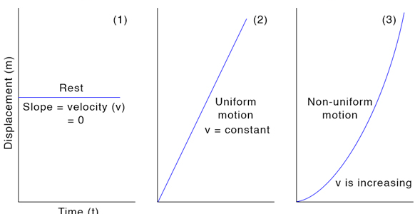
Interpretation:
- Positive slope → motion in forward direction.
- Negative slope → motion in reverse direction.
- Zero slope (flat line) → stationary object.
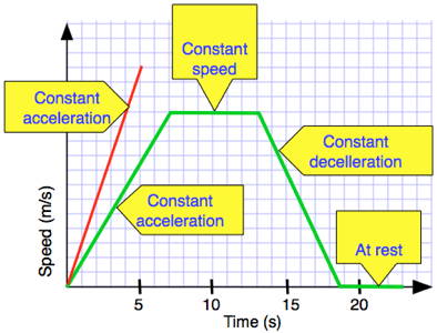
Velocity–Time Graphs
Quantity represented: Velocity (vector).
- Shows how velocity varies with time.
- The slope (gradient) represents acceleration.
- The area under the curve gives displacement.
Gradient: \( \mathrm{a = \dfrac{\Delta v}{\Delta t}} \)
Area under curve: \( \mathrm{s = \int v\,dt} \)

Interpretation:
- Positive gradient → acceleration.
- Negative gradient → deceleration.
- Zero gradient (horizontal line) → constant velocity.
Speed–Time Graphs
Quantity represented: Speed (scalar).
- Similar to a velocity–time graph but direction is ignored (always positive).
- Area under the graph gives distance travelled.
Area under curve: \( \mathrm{distance = \int v\,dt} \)
Interpretation:
- Steeper slope → faster change in speed.
- Flat line → constant speed.
Acceleration–Time Graphs
Quantity represented: Acceleration (vector).
- Shows how acceleration changes over time.
- The area under the curve gives the change in velocity.
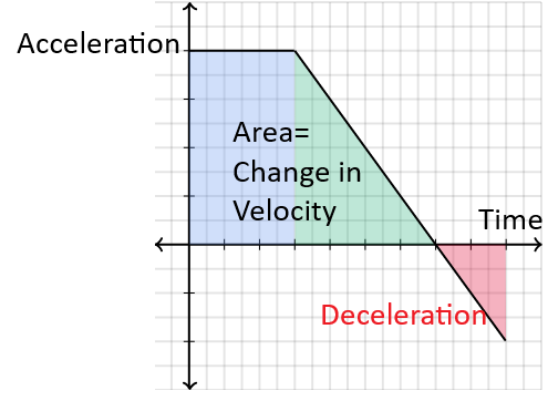
Area under curve: \( \mathrm{\Delta v = \int a\,dt} \)
Interpretation:
- Horizontal line → constant acceleration.
- Below time axis → negative acceleration (deceleration).
Relationship Summary
| Graph Type | Gradient (Slope) | Area Under Graph |
|---|---|---|
| Distance–Time | Speed | — |
| Displacement–Time | Velocity | — |
| Velocity–Time | Acceleration | Displacement |
| Speed–Time | Rate of change of speed | Distance |
| Acceleration–Time | Rate of change of acceleration (jerk) | Change in velocity |
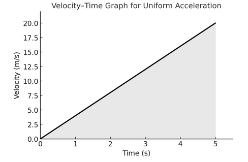
Example
A body starts from rest and accelerates uniformly to \( \mathrm{20\,m/s} \) in \( \mathrm{5\,s.} \) Find the acceleration and displacement using the velocity–time graph.
▶️ Answer / Explanation
Step 1: The v–t graph is a straight line from (0,0) to (5,20).
Acceleration (slope): \( \mathrm{a = \dfrac{\Delta v}{\Delta t} = \dfrac{20 – 0}{5 – 0} = 4.0\,m/s^2} \)
Step 2: Displacement = area under graph.
Area = area of triangle under line = \( \mathrm{\tfrac{1}{2} \times base \times height} \)
\( \mathrm{s = \tfrac{1}{2} \times 5 \times 20 = 50\,m.} \)
Result: \( \mathrm{a = 4.0\,m/s^2, \ s = 50\,m.} \)
Determining Displacement from the Area Under a Velocity–Time Graph
The area under a velocity–time (v–t) graph represents the displacement of an object. This is because the product of velocity and time gives displacement.

\( \mathrm{Displacement = \int v\,dt} \)
- In a \( \mathrm{v–t} \) graph, area under the curve = change in position.
- The sign of the area indicates direction:
- Positive area → motion in the positive direction
- Negative area → motion in the opposite direction
- If motion reverses, total displacement = (area above axis) − (area below axis).
Units:
Velocity (\( \mathrm{m/s} \)) × Time (\( \mathrm{s} \)) = Displacement (\( \mathrm{m} \))
Cases:
| Shape of v–t Graph | Calculation of Area (Displacement) |
|---|---|
| Constant velocity (horizontal line) | \( \mathrm{s = v \times t} \) |
| Uniform acceleration (straight line) | \( \mathrm{s = \tfrac{1}{2}(v + u)t} \) |
| Changing acceleration (curved line) | Area found by counting squares or using calculus: \( \mathrm{s = \int v\,dt} \) |
Example
An object moves with uniform acceleration from rest to \( \mathrm{20\,m/s} \) in \( \mathrm{4\,s} \). Find the displacement during this time.
▶️ Answer / Explanation
Step 1: Draw a straight-line v–t graph from (0, 0) to (4, 20). The area under the line = area of a triangle.
Step 2: Calculate the area.
\( \mathrm{s = \tfrac{1}{2} \times base \times height} \)
\( \mathrm{s = \tfrac{1}{2} \times 4 \times 20 = 40\,m} \)
Result: The object’s displacement in 4 seconds is \( \mathrm{40\,m.} \)
Determining Velocity Using the Gradient of a Displacement–Time Graph
The gradient (slope) of a displacement–time (s–t) graph gives the object’s velocity. This is because velocity is defined as the rate of change of displacement with respect to time.
\( \mathrm{v = \dfrac{ds}{dt}} \)
Key Idea:
- On an s–t graph, the y-axis represents displacement and the x-axis represents time.
- The steeper the slope, the greater the velocity.
- A positive slope indicates motion in the forward direction, and a negative slope indicates motion in the opposite direction.
Units:
Displacement (\( \mathrm{m} \)) ÷ Time (\( \mathrm{s} \)) = Velocity (\( \mathrm{m/s} \))
Types of Graphs and Motion:
| Shape of s–t Graph | Type of Motion | Velocity (Interpretation of Slope) |
|---|---|---|
| Straight line with constant positive slope | Uniform motion | Constant positive velocity |
| Horizontal line (zero slope) | Object at rest | Zero velocity |
| Straight line with constant negative slope | Uniform motion in opposite direction | Constant negative velocity |
| Curved line (increasing slope) | Acceleration | Velocity increasing with time |
| Curved line (decreasing slope) | Deceleration | Velocity decreasing with time |
Example
An object’s displacement–time graph is a straight line passing through points \( \mathrm{(0\,s,\,0\,m)} \) and \( \mathrm{(4\,s,\,20\,m)} \). Determine the velocity of the object.
▶️ Answer / Explanation
Step 1: The velocity is the gradient of the s–t graph.
\( \mathrm{v = \dfrac{\Delta s}{\Delta t}} \)
Step 2: Substitute values.
\( \mathrm{v = \dfrac{20 – 0}{4 – 0} = 5.0\,m/s.} \)
Step 3: Interpretation.
Constant slope → uniform velocity of \( \mathrm{5.0\,m/s.} \)
Result: The object moves with a constant velocity of \( \mathrm{5.0\,m/s} \) in the positive direction.
Determining Acceleration Using the Gradient of a Velocity–Time Graph
The gradient (slope) of a velocity–time (v–t) graph gives the object’s acceleration. This is because acceleration is the rate of change of velocity with respect to time.
\( \mathrm{a = \dfrac{\Delta v}{\Delta t}} \)
Key Idea:
- The steeper the slope, the greater the acceleration.
- A positive slope indicates acceleration in the forward direction.
- A negative slope indicates deceleration (negative acceleration).
- A horizontal line (zero slope) indicates uniform velocity (zero acceleration).
Units:
Velocity (\( \mathrm{m/s} \)) ÷ Time (\( \mathrm{s} \)) = Acceleration (\( \mathrm{m/s^2} \))
Types of v–t Graphs and Motion:
| Shape of v–t Graph | Type of Motion | Interpretation of Gradient (Acceleration) |
|---|---|---|
| Straight line with constant positive slope | Uniform acceleration | Constant positive acceleration |
| Straight line with constant negative slope | Uniform deceleration | Constant negative acceleration |
| Horizontal line (zero slope) | Uniform velocity | Zero acceleration |
| Curved line (increasing slope) | Non-uniform acceleration | Acceleration increasing with time |
| Curved line (decreasing slope) | Non-uniform deceleration | Acceleration decreasing with time |
Instantaneous Acceleration:
- If the v–t graph is curved, the acceleration is not constant.
- The acceleration at any instant is found by drawing a tangent at that point and finding its gradient.
\( \mathrm{a_{instantaneous} = \text{slope of tangent on v–t graph}} \)
Example
A car’s velocity increases from \( \mathrm{10\,m/s} \) to \( \mathrm{30\,m/s} \) in \( \mathrm{5\,s.} \) Find its acceleration.
▶️ Answer / Explanation
Step 1: Use the gradient of the v–t graph.
\( \mathrm{a = \dfrac{\Delta v}{\Delta t}} \)
Step 2: Substitute the values.
\( \mathrm{a = \dfrac{30 – 10}{5 – 0} = \dfrac{20}{5} = 4.0\,m/s^2} \)
Step 3: Interpretation.
The positive slope indicates acceleration in the forward direction.
Result: The car’s acceleration is \( \mathrm{4.0\,m/s^2.} \)
Deriving the Equations of Uniformly Accelerated Motion
When an object moves along a straight line with a constant acceleration, the motion is called uniformly accelerated motion. From the definitions of velocity and acceleration, we can derive three fundamental equations (often called the kinematic equations).
These equations relate five quantities:
- \( \mathrm{u} \): initial velocity (m/s)
- \( \mathrm{v} \): final velocity (m/s)
- \( \mathrm{a} \): constant acceleration (m/s²)
- \( \mathrm{t} \): time (s)
- \( \mathrm{s} \): displacement (m)
Starting from the Basic Definitions
Velocity: \( \mathrm{v = \dfrac{ds}{dt}} \)
Acceleration: \( \mathrm{a = \dfrac{dv}{dt}} \)
For uniform (constant) acceleration:
\( \mathrm{a = \dfrac{v – u}{t}} \)
Equation (1): \( \mathrm{v = u + at} \)
Derivation:
By definition of constant acceleration,
\( \mathrm{a = \dfrac{v – u}{t}} \)
Rearranging gives:
\( \mathrm{v = u + at} \)
Meaning: Final velocity = initial velocity + (acceleration × time).
Equation (2): \( \mathrm{s = ut + \tfrac{1}{2}at^2} \)
Derivation:
Velocity is the rate of change of displacement:
\( \mathrm{v = \dfrac{ds}{dt}} \)
From Equation (1), \( \mathrm{v = u + at} \).
Substitute into \( \mathrm{v = \dfrac{ds}{dt}} \):
\( \mathrm{\dfrac{ds}{dt} = u + at} \)
Integrate both sides from \( \mathrm{t = 0} \) to \( \mathrm{t = t} \):
\( \displaystyle \int_0^s ds = \int_0^t (u + at)\,dt \)
Integrating:
\( \mathrm{s = ut + \tfrac{1}{2}at^2} \)
Meaning: Displacement = (distance covered if moving at constant velocity \( \mathrm{u} \)) + (extra distance due to acceleration).
Equation (3): \(\mathrm{v^2 = u^2 + 2as}\)
Derivation:
From Equation (1): \( \mathrm{v = u + at} \)
and from Equation (2): \( \mathrm{s = ut + \tfrac{1}{2}at^2} \).
Eliminate \( \mathrm{t} \) between them.
From Equation (1): \( \mathrm{t = \dfrac{v – u}{a}} \)
Substitute into Equation (2):
\( \mathrm{s = u\dfrac{v – u}{a} + \tfrac{1}{2}a\left(\dfrac{v – u}{a}\right)^2} \)
Simplify:
\( \mathrm{s = \dfrac{uv – u^2}{a} + \dfrac{(v – u)^2}{2a}} \)
\( \mathrm{s = \dfrac{2uv – 2u^2 + v^2 – 2uv + u^2}{2a}} \)
\( \mathrm{s = \dfrac{v^2 – u^2}{2a}} \)
Rearranging:
\( \mathrm{v^2 = u^2 + 2as} \)
Meaning: This equation relates velocity and displacement directly, without time.
Equation (4): $\mathrm{s = \tfrac{1}{2}(u + v)t}$
Derivation (using average velocity):
For uniform acceleration, average velocity = mean of initial and final velocities:
\( \mathrm{v_{avg} = \tfrac{u + v}{2}} \)
But \( \mathrm{s = v_{avg} \times t} \).
Therefore:
\( \mathrm{s = \tfrac{1}{2}(u + v)t} \)
Meaning: Displacement = (average velocity) × (time).
Summary of the Three Core Equations of Uniformly Accelerated Motion
| Equation | Relationship | Time Present? | Use When… |
|---|---|---|---|
| \( \mathrm{v = u + at} \) | Velocity–Time | Yes | Acceleration and time are known |
| \( \mathrm{s = ut + \tfrac{1}{2}at^2} \) | Displacement–Time | Yes | Initial velocity and time are known |
| \( \mathrm{v^2 = u^2 + 2as} \) | Velocity–Displacement | No | Time is not known |
Example
A car starts from rest and accelerates uniformly at \( \mathrm{2.0\,m/s^2} \) for \( \mathrm{8.0\,s} \). Find (a) its final velocity and (b) the distance travelled.
▶️ Answer / Explanation
Given: \( \mathrm{u = 0\,m/s,\ a = 2.0\,m/s^2,\ t = 8.0\,s} \)
(a) Final velocity:
\( \mathrm{v = u + at = 0 + (2.0)(8.0) = 16\,m/s.} \)
(b) Displacement:
\( \mathrm{s = ut + \tfrac{1}{2}at^2 = 0 + \tfrac{1}{2}(2.0)(8.0)^2 = 64\,m.} \)
Result: \( \mathrm{v = 16\,m/s,\quad s = 64\,m.} \)
Solving Problems Using Equations of Uniformly Accelerated Motion
When an object moves along a straight line with a constant acceleration, the motion is described by the three kinematic equations of uniformly accelerated motion. These equations apply to all motion in a straight line including objects moving vertically under the influence of gravity, provided air resistance is neglected.
The Three Kinematic Equations
For motion with constant acceleration \( \mathrm{a} \):
- \( \mathrm{v = u + at} \)
- \( \mathrm{s = ut + \tfrac{1}{2}at^2} \)
- \( \mathrm{v^2 = u^2 + 2as} \)
where:
- \( \mathrm{u} \) = initial velocity (m/s)
- \( \mathrm{v} \) = final velocity (m/s)
- \( \mathrm{a} \) = acceleration (m/s²)
- \( \mathrm{s} \) = displacement (m)
- \( \mathrm{t} \) = time (s)
Free Fall in a Uniform Gravitational Field
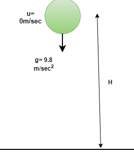
- Objects near Earth’s surface experience approximately constant acceleration due to gravity.
- This acceleration is denoted by \( \mathrm{g = 9.8\,m/s^2} \), directed downward.
- When air resistance is neglected, all objects fall at the same rate regardless of mass.
Sign convention:
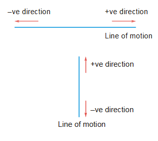
- If downward motion is taken as positive → \( \mathrm{a = +g} \)
- If upward motion is taken as positive → \( \mathrm{a = -g} \)
Key Notes and Tips for Solving Problems
- Always identify the known and unknown quantities first.
- Choose one of the three equations depending on which variable is missing.
- Maintain consistent units (m, s, m/s, m/s²).
- Remember that signs (+ or −) indicate direction — e.g., upward vs downward.
- For free-fall motion, use \( \mathrm{a = g = 9.8\,m/s^2} \) (if downward positive).
- If an object is thrown upward, its velocity at the top of the path is zero (\( \mathrm{v = 0} \)).
Summary of Situations and Equations
| Given | Find | Equation to Use |
|---|---|---|
| \( \mathrm{u, a, t} \) | \( \mathrm{v,\ s} \) | \( \mathrm{v = u + at,\ \ s = ut + \tfrac{1}{2}at^2} \) |
| \( \mathrm{u, v, s} \) | \( \mathrm{a} \) | \( \mathrm{v^2 = u^2 + 2as} \) |
| \( \mathrm{v, a, s} \) | \( \mathrm{u} \) | \( \mathrm{v^2 = u^2 + 2as} \) |
| \( \mathrm{s, u, a} \) | \( \mathrm{t} \) | \( \mathrm{s = ut + \tfrac{1}{2}at^2} \) |
Example
A car accelerates uniformly from rest at \( \mathrm{a = 3.0\,m/s^2} \) for \( \mathrm{6.0\,s} \). Find (a) its final velocity and (b) the distance covered.
▶️ Answer / Explanation
Given: \( \mathrm{u = 0,\ a = 3.0\,m/s^2,\ t = 6.0\,s.} \)
(a) Final velocity:
\( \mathrm{v = u + at = 0 + (3.0)(6.0) = 18.0\,m/s.} \)
(b) Distance travelled:
\( \mathrm{s = ut + \tfrac{1}{2}at^2 = 0 + \tfrac{1}{2}(3.0)(6.0)^2 = 54.0\,m.} \)
Result: \( \mathrm{v = 18.0\,m/s,\quad s = 54.0\,m.} \)
Example
A motorcycle increases speed from \( \mathrm{10.0\,m/s} \) to \( \mathrm{25.0\,m/s} \) over a distance of \( \mathrm{70.0\,m.} \) Find its acceleration.
▶️ Answer / Explanation
Given: \( \mathrm{u = 10.0\,m/s,\ v = 25.0\,m/s,\ s = 70.0\,m.} \)
Use: \( \mathrm{v^2 = u^2 + 2as} \Rightarrow \mathrm{a = \dfrac{v^2 – u^2}{2s}} \)
\( \mathrm{a = \dfrac{25.0^2 – 10.0^2}{2(70)} = \dfrac{625 – 100}{140} = \dfrac{525}{140} = 3.75\,m/s^2.} \)
Result: The motorcycle accelerates at \( \mathrm{3.75\,m/s^2.} \)
Example
A stone is dropped from a height of \( \mathrm{50.0\,m.} \) Neglecting air resistance, find (a) the time taken to reach the ground and (b) its impact speed. Take \( \mathrm{g = 9.8\,m/s^2.} \)
▶️ Answer / Explanation
Given: \( \mathrm{u = 0\,m/s,\ s = 50.0\,m,\ a = g = 9.8\,m/s^2.} \)
(a) Time to fall:
\( \mathrm{s = ut + \tfrac{1}{2}at^2 \Rightarrow 50.0 = 0 + 0.5(9.8)t^2} \)
\( \mathrm{t^2 = \dfrac{50.0\times2}{9.8} = 10.204} \Rightarrow t = 3.19\,s.} \)
(b) Final velocity:
\( \mathrm{v = u + at = 0 + 9.8(3.19) = 31.3\,m/s.} \)
Result: Time to hit ground = \( \mathrm{3.19\,s} \); impact velocity = \( \mathrm{31.3\,m/s\ (downward)}. \)
Experiment to determine the acceleration of free fall ( \( \mathrm{g} \) ) using a falling object
Aim:
To determine the acceleration due to free fall \( \mathrm{g} \) by measuring the time taken for an object to fall through known vertical distances and using the kinematic relation for motion from rest.
Apparatus: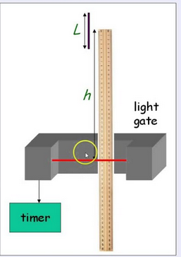
- Rigid clamp stand and boss
- Release mechanism (electromagnetic or simple trap that gives repeatable release)
- Photogate(s) or electronic timing gate and digital timer (preferred) — OR: a good precision stopwatch if photogates are not available
- Steel ball or small dense sphere (to reduce air resistance)
- Rule or meter stick (millimetre scale) for measuring drop height
- Measuring tape or vernier calliper for better precision of heights
- Protractor / spirit level (to ensure vertical alignment)
- Data sheet and calculator
Principle / Theory:
For an object released from rest and allowed to fall freely (neglecting air resistance), the displacement \( \mathrm{s} \) after time \( \mathrm{t} \) is given by
\( \mathrm{ s = \tfrac{1}{2} g t^2 } \)
Rearranging to solve for \( \mathrm{g} \):
\( \mathrm{ g = \dfrac{2s}{t^2} } \)
Measure \( \mathrm{s} \) and \( \mathrm{t} \) for several values of \( \mathrm{s} \); compute \( \mathrm{g} \) for each and take a mean. Use uncertainty propagation to estimate the uncertainty in \( \mathrm{g} \).
Procedure (using a single photogate / timer method):
- Fix the release mechanism at a vertical position so the ball can be released without initial push. Align the photogate a small distance below the release position if using a single photogate, or use two photogates (one near release and one at measured height) to start/stop timing automatically.
- Measure and record a set of drop heights \( \mathrm{s} \) (for example: \( \mathrm{0.50\,m,\ 1.00\,m,\ 1.50\,m,\ 2.00\,m} \)). Record each height to the best possible precision (e.g., \( \mathrm{\pm 0.005\,m} \)).
- For each height: position the lower photogate (or mark the impact point), release the ball and record the time \( \mathrm{t} \) taken to fall through distance \( \mathrm{s} \). Repeat each measurement at least 5 times to reduce random error and obtain an average time \( \overline{t} \).
- Calculate \( \mathrm{g} \) for each height using \( \mathrm{ g = \dfrac{2s}{\overline{t}^2} } \).
- Calculate the mean \( \mathrm{\langle g \rangle} \) and the uncertainty (see below). Discuss systematic and random errors and suggest improvements.
Procedure (if only stopwatch is available):
- Same idea, but human reaction time introduces a large timing uncertainty. To reduce this, perform many repeats and/or use the two-person method (one person releases, the other times) and then correct for average reaction delay if known.
Data table (template)
| Run | Drop height \( \mathrm{s} \) (m) | Trial times \( \mathrm{t_i} \) (s) | Mean \( \overline{t} \) (s) | Computed \( g = \dfrac{2s}{\overline{t}^2} \) (m/s\(^2\)) |
|---|---|---|---|---|
| 1 | 0.50 | 0.320, 0.319, 0.321, … | 0.320 | 9.80 |
| 2 | 1.00 | 0.452, 0.451, 0.453, … | 0.452 | 9.80 |
| 3 | 1.50 | 0.553, 0.552, 0.554, … | 0.553 | 9.80 |
| 4 | 2.00 | 0.639, 0.638, 0.639, … | 0.639 | 9.80 |
Sample numerical calculation & uncertainty estimation (worked example)
Take one example height: \( \mathrm{s = 1.00\,m} \). Suppose the measured mean time is \( \mathrm{\overline{t} = 0.452\,s} \). Use measurement uncertainties \( \mathrm{\Delta s = 0.005\,m} \) (±5 mm) and \( \mathrm{\Delta t = 0.002\,s} \) (timing gate precision ≈ 2 ms).
Calculate \( \mathrm{g} \):
\( \mathrm{ g = \dfrac{2s}{\overline{t}^2} = \dfrac{2(1.00)}{(0.452)^2} = 9.80\ \text{m/s}^2. } \)
Estimate the uncertainty in \( \mathrm{g} \) by adding fractional uncertainties (suitable for this syllabus):
Fractional uncertainty in \( \mathrm{s} \): \( \mathrm{\dfrac{\Delta s}{s} = \dfrac{0.005}{1.00} = 0.005 = 0.5\% } \)
Fractional uncertainty in \( \mathrm{t} \): \( \mathrm{\dfrac{\Delta t}{t} = \dfrac{0.002}{0.452} \approx 0.00442 = 0.442\% } \)
Since \( \mathrm{g = 2s t^{-2}} \), the fractional uncertainty in \( \mathrm{g} \) ≈ \( \mathrm{\dfrac{\Delta g}{g} = \dfrac{\Delta s}{s} + 2\dfrac{\Delta t}{t} } \).
Compute: \( \mathrm{\dfrac{\Delta g}{g} = 0.005 + 2(0.00442) = 0.005 + 0.00884 = 0.01384 } \) → \( \mathrm{1.384\% } \).
Absolute uncertainty: \( \mathrm{\Delta g = g \times 0.01384 = 9.80 \times 0.01384 \approx 0.14\ \text{m/s}^2 } \).
Result (example): \( \mathrm{g = (9.80 \pm 0.14)\,m/s^2} \).
Analysis & presentation:
- Calculate \( \mathrm{g} \) for each height and list them. Compute the mean \( \mathrm{\langle g \rangle} \) and the standard deviation (or standard deviation of the mean) to quote a combined experimental uncertainty.
- Plot \( \mathrm{s} \) versus \( \mathrm{t^2} \). From theory \( \mathrm{s = \tfrac{1}{2} g t^2} \) so this should be linear with slope \( \mathrm{m = \tfrac{1}{2} g} \). Fit a straight line and find slope \( \mathrm{m} \) → then \( \mathrm{g = 2m} \). This graphical method reduces influence of single-point outliers and is recommended for A Level reporting.
Improvements / extensions:
- Use two photogates and measure time between them for different separations — reduces dependence on release timing.
- Use a high-speed camera and video analysis (frame-by-frame) to get position vs time and fit \( \mathrm{s} = \tfrac{1}{2} g t^2 \) by regression.
- Use multiple heights and perform a linear fit of \( \mathrm{s} \) vs \( \mathrm{t^2} \) to find \( \mathrm{g} \) more reliably.
- Use vacuum chamber for very precise experiments to remove air resistance (advanced).
Conclusion:
Using repeated measurements of fall time for known drop heights and the relation \( \mathrm{ g = \dfrac{2s}{t^2} } \), you can determine \( \mathrm{g} \) with reasonable accuracy. Electronic timing (photogates) and plotting \( \mathrm{s} \) vs \( \mathrm{t^2} \) give the best classroom results and allow clear estimation of random and systematic uncertainties.
Motion Due to a Uniform Velocity in One Direction and a Uniform Acceleration in a Perpendicular Direction
When an object moves such that it has a constant (uniform) velocity in one direction and a uniform acceleration in a direction perpendicular to that velocity, its motion combines these two effects — resulting in a curved path (usually parabolic).
Key Idea:
- The horizontal motion is at a constant velocity (no horizontal acceleration).
- The vertical motion is uniformly accelerated (usually due to gravity).
- The combined motion produces a two-dimensional trajectory — e.g. a projectile path.
Projectile Motion
Projectile motion is the motion of an object that is projected into the air and moves under the influence of gravity alone, assuming that air resistance is negligible. The only force acting on the projectile after it is launched is its weight, producing a constant downward acceleration equal to the acceleration due to gravity \( \mathrm{g} \).
Nature of Motion:
The motion of a projectile is two-dimensional. It can be analysed as two independent components of motion:
- Horizontal motion — with uniform velocity (no horizontal acceleration)
- Vertical motion — with uniform acceleration (acceleration due to gravity)
These two motions occur simultaneously and combine to form a curved trajectory known as a parabolic path.
Assumptions:
- Air resistance is negligible.
- The acceleration due to gravity \( \mathrm{g} \) is constant and acts vertically downward.
- The effect of Earth’s rotation is neglected.
Resolution of Initial Velocity:
If a projectile is launched with an initial velocity \( \mathrm{u} \) at an angle \( \mathrm{\theta} \) to the horizontal:
Horizontal component: \( \mathrm{u_x = u\cos\theta} \)
Vertical component: \( \mathrm{u_y = u\sin\theta} \)
Equations of Motion:
The horizontal and vertical motions are treated separately using the equations of uniformly accelerated motion.
Horizontal Motion:
- Acceleration \( \mathrm{a_x = 0} \)
- Velocity remains constant: \( \mathrm{v_x = u_x = u\cos\theta} \)
- Displacement after time \( \mathrm{t} \): \( \mathrm{x = u_x t = (u\cos\theta)t} \)
Vertical Motion:
- Acceleration \( \mathrm{a_y = -g} \) (downward)
- Velocity after time \( \mathrm{t} \): \( \mathrm{v_y = u_y – gt = u\sin\theta – gt} \)
- Vertical displacement after time \( \mathrm{t} \): \( \mathrm{y = u_y t – \tfrac{1}{2}gt^2 = (u\sin\theta)t – \tfrac{1}{2}gt^2} \)
Equation of Trajectory:
From horizontal motion, \( \mathrm{t = \dfrac{x}{u\cos\theta}} \)
Substituting in the vertical displacement equation gives:
\( \mathrm{y = x\tan\theta – \dfrac{g x^2}{2u^2 \cos^2\theta}} \)
This is the general equation of a parabola, showing that the path of a projectile is parabolic.
Time of Flight:
The total time the projectile remains in the air before returning to the same vertical level as the launch point is given by:
\( \mathrm{T = \dfrac{2u\sin\theta}{g}} \)
Maximum Height:
The greatest vertical displacement reached by the projectile occurs when the vertical velocity becomes zero \( \mathrm{(v_y = 0)} \).
\( \mathrm{H = \dfrac{u^2\sin^2\theta}{2g}} \)
Horizontal Range:
The horizontal distance travelled by the projectile during the total time of flight is called the range.
\( \mathrm{R = u_x T = \dfrac{u^2\sin(2\theta)}{g}} \)
Key Features of Projectile Motion:
- The horizontal component of velocity remains constant throughout the motion.
- The vertical component of velocity changes uniformly under gravity.
- The path of the projectile is parabolic.
- The maximum range occurs when \( \mathrm{\theta = 45^\circ} \).
- Time of ascent = time of descent (for motion returning to the same vertical level).
- At the highest point, vertical velocity is zero, but horizontal velocity remains constant.
Summary of Main Equations:
| Quantity | Expression |
|---|---|
| Horizontal displacement | \( \mathrm{x = u\cos\theta \, t} \) |
| Vertical displacement | \( \mathrm{y = u\sin\theta \, t – \tfrac{1}{2}gt^2} \) |
| Equation of trajectory | \( \mathrm{y = x\tan\theta – \dfrac{g x^2}{2u^2 \cos^2\theta}} \) |
| Time of flight | \( \mathrm{T = \dfrac{2u\sin\theta}{g}} \) |
| Maximum height | \( \mathrm{H = \dfrac{u^2\sin^2\theta}{2g}} \) |
| Horizontal range | \( \mathrm{R = \dfrac{u^2\sin(2\theta)}{g}} \) |
Example
A small ball rolls horizontally off a table with a speed of \( \mathrm{2.0\,m/s} \). The height of the table is \( \mathrm{1.25\,m} \). Find (a) the time taken to reach the ground, and (b) the horizontal distance travelled.
▶️ Answer / Explanation
Step 1: Vertical motion: \( \mathrm{u_y = 0}, \ a_y = g = 9.8\,m/s^2, \ s_y = 1.25\,m.} \)
Use \( \mathrm{s_y = \tfrac{1}{2} g t^2} \):
\( \mathrm{1.25 = \tfrac{1}{2}(9.8)t^2} \Rightarrow t^2 = \dfrac{2(1.25)}{9.8} = 0.255} \)
\( \mathrm{t = 0.505\,s.} \)
Step 2: Horizontal motion (constant velocity): \( \mathrm{x = u_x t = (2.0)(0.505) = 1.01\,m.} \)
Result:
- Time of flight = \( \mathrm{0.505\,s} \)
- Horizontal range = \( \mathrm{1.01\,m} \)
Path shape: Parabolic (due to uniform velocity in x, uniform acceleration in y).