Deformation Due to Tensile and Compressive Forces
Deformation occurs when forces act on a material and cause a change in its shape or length. The deformation can be either tensile (stretching) or compressive (squeezing).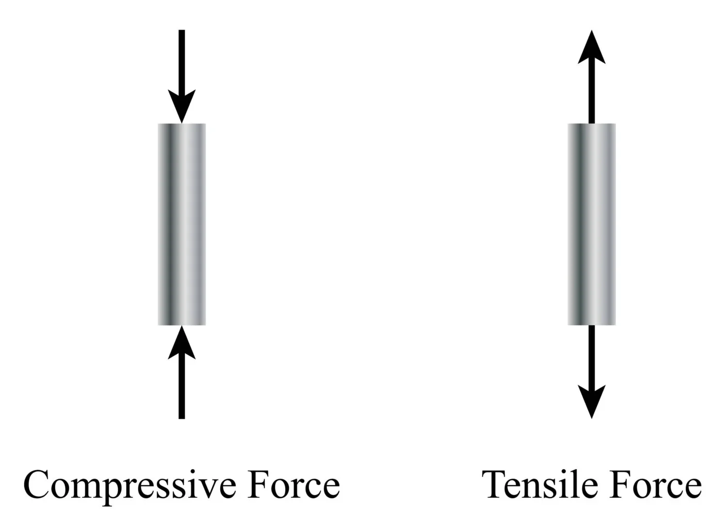
Types of Deformation:
- Tensile deformation: When equal and opposite forces act outwards on a material, increasing its length. Example: stretching a spring or wire.
- Compressive deformation: When equal and opposite forces act inwards on a material, reducing its length. Example: compressing a spring or a column under load.
Key Idea:
Both types of deformation produce changes in length that are directly proportional to the applied force, as long as the force does not exceed the limit of proportionality.
Assumption (for A Level):
All forces and deformations are assumed to act along a single straight line (one dimension). This simplifies analysis — we only consider change in length, not shape or volume.
Example
A spring is hung vertically and a 2 N weight is attached, causing it to extend. Describe the forces and type of deformation involved. What would happen if the spring were instead compressed by 2 N?
▶️ Answer / Explanation
The spring experiences tensile deformation because the weight pulls it downward, stretching it. The restoring elastic force in the spring acts upward. If compressed by 2 N, it would experience compressive deformation — its length would decrease.
Terms: Load, Extension, Compression, and Limit of Proportionality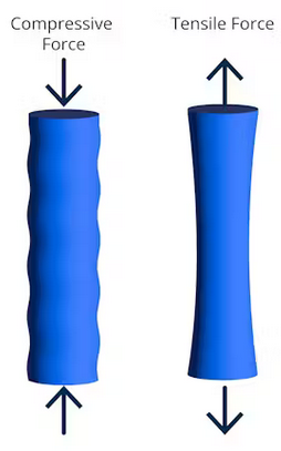
Load:
The applied force causing deformation. It can be tensile (pulling) or compressive (pushing). Unit: newton (N).
Extension (\( \mathrm{x} \)):
The increase in length of an object under a tensile load. \( \mathrm{x = l – l_0} \) where \( \mathrm{l_0} \) is original length and \( \mathrm{l} \) is stretched length.
Compression:
The decrease in length under a compressive load. It is treated as a negative extension (shortening of material).
Limit of Proportionality:

The maximum load for which the extension (or compression) is directly proportional to the applied force. Beyond this point, Hooke’s Law no longer holds — the graph of \( \mathrm{F} \) vs \( \mathrm{x} \) curves.
Graphical Representation:
- Straight line → proportional region (Hooke’s Law obeyed).
- Non-linear region → material still elastic but not proportional.
- Plastic deformation → permanent change in shape.
Example
A metal wire of original length \( \mathrm{1.5\,m} \) is stretched to \( \mathrm{1.5003\,m} \) by a 6 N load. If the graph of force vs extension begins to curve at 8 N, determine the extension at the limit of proportionality and describe what happens if the force is increased beyond this value.
▶️ Answer / Explanation
The extension under 6 N = \( \mathrm{1.5003 – 1.5 = 0.0003\,m.} \) Assuming proportional behaviour, extension increases linearly with load:
\( \mathrm{x_8 = \dfrac{8}{6} \times 0.0003 = 0.0004\,m.} \)
Beyond 8 N, the extension increases more rapidly and is no longer proportional to force — Hooke’s Law is violated.
Hooke’s Law
Statement:
Within the limit of proportionality, the extension (or compression) of a material is directly proportional to the applied force.
\( \mathrm{F \propto x} \Rightarrow \mathrm{F = kx} \)
- \( \mathrm{F} \): applied force (N)
- \( \mathrm{x} \): extension or compression (m)
- \( \mathrm{k} \): spring constant or stiffness (N·m⁻¹)
Interpretation:
- The constant \( \mathrm{k} \) measures how stiff the spring or material is — a larger \( \mathrm{k} \) means a stiffer material.
- The linear relationship holds until the limit of proportionality is reached.
- The line on an \( \mathrm{F\text{–}x} \) graph passes through the origin with slope equal to \( \mathrm{k.} \)
SI Unit of \( \mathrm{k} \): \( \mathrm{N·m^{-1}} \)
Combined Springs:
- Series: \( \mathrm{\dfrac{1}{k_{eq}} = \dfrac{1}{k_1} + \dfrac{1}{k_2}} \)
- Parallel: \( \mathrm{k_{eq} = k_1 + k_2} \)
Example
A spring extends by \( \mathrm{0.04\,m} \) when a force of \( \mathrm{8.0\,N} \) is applied. Determine the spring constant and the force required to produce an extension of \( \mathrm{0.06\,m.} \)
▶️ Answer / Explanation
Using \( \mathrm{F = kx,} \)
\( \mathrm{k = \dfrac{F}{x} = \dfrac{8.0}{0.04} = 200\,N·m^{-1}.} \)
For \( \mathrm{x = 0.06\,m:} \)
\( \mathrm{F = kx = 200 \times 0.06 = 12\,N.} \)
The spring constant is \( \mathrm{200\,N·m^{-1}} \), and the required force is \( \mathrm{12\,N.} \)
Formula for the Spring Constant
The spring constant (or force constant) \( \mathrm{k} \) measures how stiff a spring or wire is. It relates the applied force to the extension produced within the limit of proportionality.
Formula:
\( \mathrm{k = \dfrac{F}{x}} \)
- \( \mathrm{k} \): spring constant (N·m⁻¹)
- \( \mathrm{F} \): applied force (N)
- \( \mathrm{x} \): extension or compression (m)
Interpretation:
- Large \( \mathrm{k} \) → stiffer material (small extension for a given load).
- Small \( \mathrm{k} \) → more easily stretched material.
- The gradient of the \( \mathrm{F\text{–}x} \) graph in the linear region gives \( \mathrm{k.} \)
Units:
\( \mathrm{1\,N·m^{-1} = 1\,N / 1\,m.} \)
Example
A spring extends by \( \mathrm{0.050\,m} \) when a \( \mathrm{10.0\,N} \) force is applied. Calculate the spring constant.
▶️ Answer / Explanation
Using \( \mathrm{k = \dfrac{F}{x}} \):
\( \mathrm{k = \dfrac{10.0}{0.050} = 200\,N·m^{-1}.} \)
The spring constant is \( \mathrm{200\,N·m^{-1}.} \)
Stress, Strain, and the Young Modulus
(a) Stress \(( \mathrm{\sigma} )\)
Stress is the force applied per unit cross-sectional area of the material.
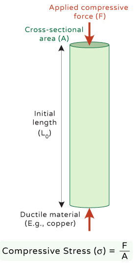
\( \mathrm{\sigma = \dfrac{F}{A}} \)
- \( \mathrm{\sigma} \): stress (Pa or N·m⁻²)
- \( \mathrm{F} \): applied force (N)
- \( \mathrm{A} \): cross-sectional area (m²)
Example
A copper wire of diameter \( \mathrm{1.20\,mm} \) is subjected to a load of \( \mathrm{15.0\,N.} \) Calculate the stress in the wire.
▶️ Answer / Explanation
Step 1: Calculate the cross-sectional area:
\( \mathrm{A = \dfrac{\pi d^2}{4} = \dfrac{\pi (1.20\times10^{-3})^2}{4} = 1.13\times10^{-6}\,m^2.} \)
Step 2: Calculate stress:
\( \mathrm{\sigma = \dfrac{F}{A} = \dfrac{15.0}{1.13\times10^{-6}} = 1.33\times10^{7}\,Pa.} \)
Step 3: Final Answer:
The stress in the wire is \( \mathrm{1.3\times10^{7}\,Pa} \) (or \( \mathrm{13\,MPa.} \))
(b) Strain \(( \mathrm{\varepsilon} )\)
Strain is the fractional change in length of the material.
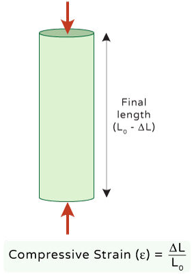
\( \mathrm{\varepsilon = \dfrac{\Delta L}{L_0}} \)
- \( \mathrm{\varepsilon} \): strain (no units — it’s a ratio)
- \( \mathrm{\Delta L} \): extension (m)
- \( \mathrm{L_0} \): original length (m)
Example
A steel wire of original length \( \mathrm{1.50\,m} \) stretches by \( \mathrm{0.60\,mm} \) when loaded. Find the strain in the wire.
▶️ Answer / Explanation
Step 1: Convert all units to metres:
\( \mathrm{L_0 = 1.50\,m, \; \Delta L = 0.60\,mm = 0.60\times10^{-3}\,m.} \)
Step 2: Apply the strain formula:
\( \mathrm{\varepsilon = \dfrac{\Delta L}{L_0} = \dfrac{0.60\times10^{-3}}{1.50} = 4.0\times10^{-4}.} \)
Step 3: Final Answer:
The strain in the wire is \( \mathrm{4.0\times10^{-4}} \) (dimensionless).
(c) Young’s Modulus \(( \mathrm{E} )\)
Young’s modulus is the ratio of tensile stress to tensile strain, for a material within its limit of proportionality.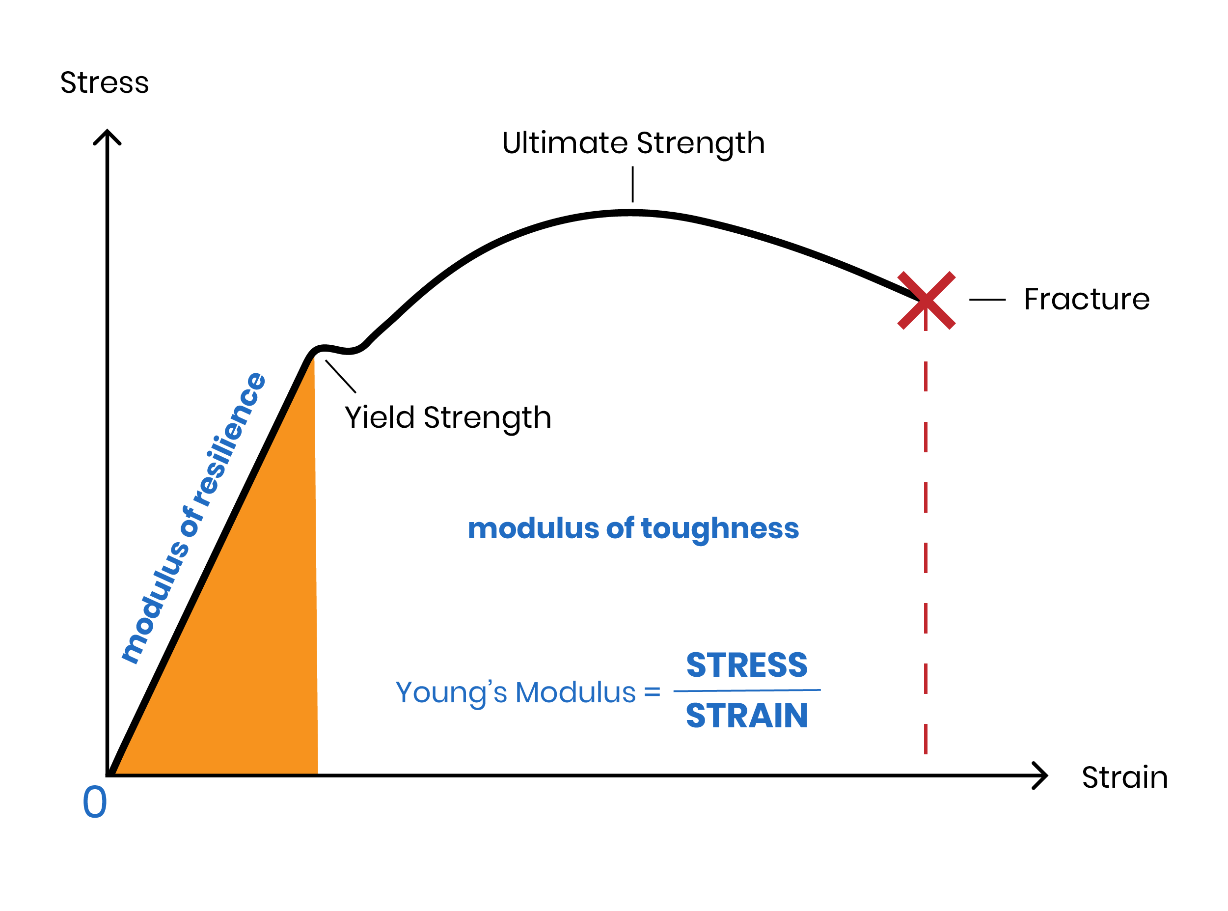
\( \mathrm{E = \dfrac{\sigma}{\varepsilon} = \dfrac{F L_0}{A \Delta L}} \)
- \( \mathrm{E} \): Young’s modulus (Pa or N·m⁻²)
- \( \mathrm{F} \): applied force (N)
- \( \mathrm{L_0} \): original length (m)
- \( \mathrm{A} \): cross-sectional area (m²)
- \( \mathrm{\Delta L} \): extension (m)
Interpretation:
- Large \( \mathrm{E} \): material is stiff — small strain for given stress.
- Small \( \mathrm{E} \): material is flexible — large strain for given stress.
- Unit of \( \mathrm{E} \): Pascal (Pa), where \( \mathrm{1\,Pa = 1\,N·m^{-2}.} \)
Example
A steel wire of original length \( \mathrm{2.0\,m} \) and cross-sectional area \( \mathrm{1.0\times10^{-6}\,m^2} \) extends by \( \mathrm{1.0\,mm} \) when a force of \( \mathrm{20\,N} \) is applied. Calculate the Young’s modulus of the steel wire.
▶️ Answer / Explanation
Given: \( \mathrm{F = 20\,N, \, A = 1.0\times10^{-6}\,m^2, \, L_0 = 2.0\,m, \, \Delta L = 1.0\times10^{-3}\,m.} \)
Using \( \mathrm{E = \dfrac{F L_0}{A \Delta L}} \):
\( \mathrm{E = \dfrac{20 \times 2.0}{(1.0\times10^{-6})(1.0\times10^{-3})} = 4.0\times10^{10}\,Pa.} \)
The Young’s modulus of the steel wire = \( \mathrm{4.0\times10^{10}\,Pa.} \)
Experimental Determination of the Young’s Modulus (for a Wire)
Objective:
To determine the Young’s modulus \( \mathrm{E} \) of a metal wire by measuring its extension under different loads.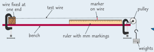
Apparatus:
- Metal wire (e.g., copper or steel) of uniform cross-section
- Fixed support (clamp stand)
- Micrometer screw gauge (for wire diameter)
- Metre rule or vernier scale (for extension)
- Weights or hanger (for load)
- Pointer or marker attached to wire (to measure small extensions)
Procedure:
- Secure the wire vertically between a fixed support and a weight hanger.
- Measure the original length \( \mathrm{L_0} \) between the fixed point and the marker.
- Measure the diameter \( \mathrm{d} \) of the wire at several points and average to calculate the cross-sectional area \( \mathrm{A = \dfrac{\pi d^2}{4}}. \)
- Add known masses incrementally to the hanger, recording the corresponding extension \( \mathrm{\Delta L} \) for each load.
- Plot a graph of \(\mathrm{F}\) (on the y-axis) against \(\mathrm{\Delta L}\) (on the x-axis).
- The straight-line portion obeys Hooke’s Law.
- The gradient \( \mathrm{= \dfrac{F}{\Delta L}}. \)
- Determine the Young’s modulus using:
- \( \mathrm{E = \dfrac{L_0}{A} \times \text{gradient of } (F \text{ vs } \Delta L).} \)
Precautions:
- Ensure the wire is free of kinks and measured under small initial tension to remove slack.
- Measure extensions after allowing the wire to stop oscillating.
- Keep loads within the proportional limit (avoid permanent deformation).
- Record diameter at multiple points to reduce random errors.
Graph and Analysis:
The graph of \( \mathrm{F} \) vs \( \mathrm{\Delta L} \) is linear within the elastic limit.
- Slope \( \mathrm{= \dfrac{F}{\Delta L}}. \)
- Using \( \mathrm{E = \dfrac{F L_0}{A \Delta L}} \),
\( \mathrm{E = \dfrac{L_0}{A} \times \text{slope of } (F\text{–}\Delta L) \text{ graph}.} \)
Example
A steel wire of diameter \( \mathrm{0.50\,mm} \) and length \( \mathrm{1.5\,m} \) extends by \( \mathrm{0.45\,mm} \) under a load of \( \mathrm{5.0\,N.} \) Calculate the Young’s modulus.
▶️ Answer / Explanation
Given: \( \mathrm{d = 0.50\,mm = 0.50\times10^{-3}\,m, \; A = \dfrac{\pi d^2}{4} = 1.96\times10^{-7}\,m^2,} \) \( \mathrm{L_0 = 1.5\,m, \; \Delta L = 0.45\times10^{-3}\,m, \; F = 5.0\,N.} \)
Using \( \mathrm{E = \dfrac{F L_0}{A \Delta L}} \):
\( \mathrm{E = \dfrac{5.0 \times 1.5}{(1.96\times10^{-7})(0.45\times10^{-3})} = 8.5\times10^{10}\,Pa.} \)
The Young’s modulus of the steel wire ≈ \( \mathrm{8.5\times10^{10}\,Pa.} \)