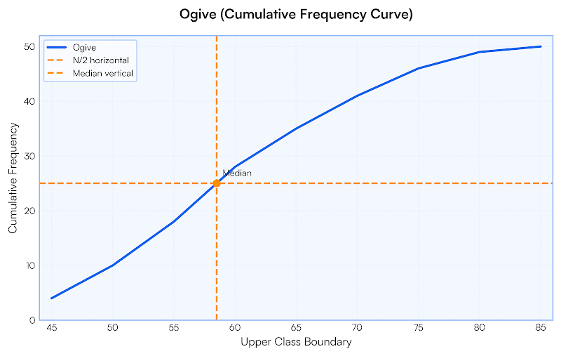
Estimating the Median from a Cumulative Frequency Diagram
A cumulative frequency diagram (often called an ogive) shows the total number of values up to a given point.
We use it to estimate the median, which is the middle value of the data.
Step-by-Step Method
- Find the total frequency (the highest value on the cumulative frequency axis).
- Divide this by 2 to locate the middle value.
- From this number, draw a horizontal line across to the curve.
- From where it meets the curve, draw a vertical line down to the horizontal axis.
- The value on the horizontal axis is the estimated median.
Important Idea
Because the data is grouped, the median is only an estimate.
The median splits the data into two equal halves.
Example 1:
A cumulative frequency graph shows a total frequency of 80. Estimate the median position.
▶️ Answer/Explanation
Median position \( =\dfrac{80}{2}=40 \)
Conclusion: Read the value corresponding to cumulative frequency 40.
Example 2:
The total number of students is 120. At what cumulative frequency should you read the median?
▶️ Answer/Explanation
Median position \( =\dfrac{120}{2}=60 \)
Conclusion: Read from cumulative frequency 60.
Example 3:
Explain why the median is not exact when using a cumulative frequency diagram.
▶️ Answer/Explanation
The data is grouped into class intervals.
We read a value from a smooth curve.
Conclusion: Therefore the median is an estimate.
Measure of Spread
An average (mean, median or mode) tells us the centre of the data.
However, it does not tell us how spread out the data values are.
A measure of spread describes how much the data varies.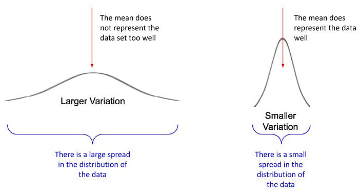
Why It Matters
Two data sets can have the same mean but be very different.
- Small spread → values close together
- Large spread → values widely scattered
Common Measure of Spread
The most basic measure of spread is the range.
\( \text{Range}=\text{highest value}-\text{lowest value} \)
A small range means consistent data. A large range means inconsistent data.
Key Idea
When comparing two groups, we consider both:
- Average (centre)
- Spread (variation)
Example 1:
Find the range of the data set: \( 4,\;6,\;7,\;8,\;10 \).
▶️ Answer/Explanation
Highest \( =10 \)
Lowest \( =4 \)
Range \( =10-4=6 \)
Conclusion: Range \( =6 \).
Example 2:
Two classes both have mean score 60. Class A scores: 58, 59, 60, 61, 62 Class B scores: 20, 40, 60, 80, 100 Which class is more consistent?
▶️ Answer/Explanation
Find ranges.
Class A: \( 62-58=4 \)
Class B: \( 100-20=80 \)
Conclusion: Class A is more consistent (smaller spread).
Example 3:
Explain why average alone is not enough to compare data sets.
▶️ Answer/Explanation
Different spreads can produce the same average.
Conclusion: We must also consider variation.
Interquartile Range from a Discrete Data Set
The interquartile range (IQR) is a measure of spread.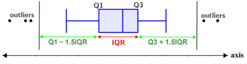
It shows how spread out the middle half of the data is.
Instead of using the smallest and largest values (like the range), the IQR ignores extreme values.
Quartiles
- Lower quartile (Q₁) → 25% of data below it
- Median (Q₂) → middle value
- Upper quartile (Q₃) → 75% of data below it
Formula
\( \text{IQR}=Q_3-Q_1 \)
Steps to Find the IQR
- Write the data in order (smallest to largest)
- Find the median
- Find the median of the lower half → \( Q_1 \)
- Find the median of the upper half → \( Q_3 \)
- Subtract \( Q_1 \) from \( Q_3 \)
Important Idea
The IQR measures consistency.
- Small IQR → values close together
- Large IQR → values spread out
Example 1:
Find the IQR of: \( 2,\;4,\;5,\;6,\;7,\;8,\;10 \).
▶️ Answer/Explanation
Median \( =6 \)
Lower half: \( 2,4,5 \) → \( Q_1=4 \)
Upper half: \( 7,8,10 \) → \( Q_3=8 \)
\( \text{IQR}=8-4=4 \)
Conclusion: IQR \( =4 \).
Example 2:
Find \( Q_1 \) and \( Q_3 \) for: \( 3,\;5,\;6,\;7,\;9,\;11,\;13,\;15 \).
▶️ Answer/Explanation
Median between 7 and 9.
Lower half: \( 3,5,6,7 \)
\( Q_1=\dfrac{5+6}{2}=5.5 \)
Upper half: \( 9,11,13,15 \)
\( Q_3=\dfrac{11+13}{2}=12 \)
Conclusion: \( Q_1=5.5,\;Q_3=12 \).
Example 3:
The lower quartile is 12 and the upper quartile is 20. Find the interquartile range.
▶️ Answer/Explanation
\( \text{IQR}=20-12=8 \)
Conclusion: IQR \( =8 \).
Estimating the Interquartile Range from a Cumulative Frequency Diagram
A cumulative frequency diagram can also be used to estimate the interquartile range (IQR).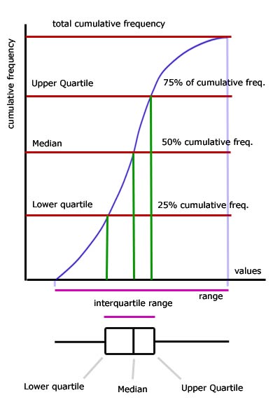
Remember:
\( \text{IQR}=Q_3-Q_1 \)
So we must find the lower quartile and upper quartile from the graph.
Steps
- Find the total frequency (highest cumulative frequency).
- Calculate \( \dfrac{1}{4} \) of the total → this gives \( Q_1 \) position.
- Calculate \( \dfrac{3}{4} \) of the total → this gives \( Q_3 \) position.
- From each value, draw a horizontal line to the curve.
- Drop a vertical line to the horizontal axis to read the data value.
- Subtract to find the IQR.
Quartile Positions
- \( Q_1=\dfrac{1}{4}\times\text{total frequency} \)
- \( Q_3=\dfrac{3}{4}\times\text{total frequency} \)
Important Idea
The IQR represents the spread of the middle 50% of the data.
Example 1:
A cumulative frequency graph has total frequency 80. Find the positions of \( Q_1 \) and \( Q_3 \).
▶️ Answer/Explanation
\( Q_1=\dfrac{1}{4}\times80=20 \)
\( Q_3=\dfrac{3}{4}\times80=60 \)
Conclusion: Read values at cumulative frequencies 20 and 60.
Example 2:
The total number of observations is 120. At what cumulative frequency do you read the upper quartile?
▶️ Answer/Explanation
\( Q_3=\dfrac{3}{4}\times120=90 \)
Conclusion: Read from cumulative frequency 90.
Example 3:
From a cumulative frequency graph you read: \( Q_1=18 \) and \( Q_3=42 \). Find the interquartile range.
▶️ Answer/Explanation
\( \text{IQR}=42-18=24 \)
Conclusion: IQR \( =24 \).