Graphical Solution of Two-Variable Linear Programming Problems
When a linear programming problem involves two decision variables, it can be solved graphically. This involves plotting the constraints on a coordinate plane and identifying the point that optimises the objective function.
Two standard graphical approaches are used:
- The ruler (objective line) method
- The vertex (corner point) method
Step 1: Plotting the Constraints
Each constraint is written as an equation to draw its boundary line.
For example, the constraint
\( \mathrm{2x + y \leq 8} \)
is plotted by drawing the line
\( \mathrm{2x + y = 8} \)
The feasible side of the line is identified using a test point, usually the origin.
Feasible Region
The feasible region is the set of all points that satisfy:
- All constraints
- Non-negativity conditions \( \mathrm{x \geq 0,\; y \geq 0} \)
Only points inside this region are valid solutions.
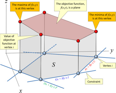
Vertex (Corner Point) Method
The vertex method is based on the fact that the optimum value of a linear objective function occurs at a vertex of the feasible region.
Procedure:
- Identify all vertices of the feasible region
- Substitute each vertex into the objective function
- Choose the vertex giving the maximum or minimum value
This method is systematic and is preferred in examinations.
Ruler (Objective Line) Method
In the ruler method, the objective function is treated as a straight line.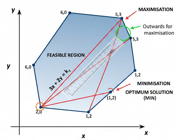
For example,
\( \mathrm{Z = 3x + 2y} \)
is rewritten as
\( \mathrm{3x + 2y = k} \)
A ruler is used to slide this line parallel across the feasible region:
- Outwards for maximisation
- Inwards for minimisation
The last point of contact with the feasible region gives the optimum solution.
Unbounded and No-Solution Cases
Unbounded solution:
The feasible region is open and the objective function increases without limit
No feasible solution:
The constraints do not overlap
Key Examination Points
- Always shade the feasible region clearly
- Label all vertices accurately
- State the optimal value and where it occurs
- Mention if the solution is unbounded or infeasible
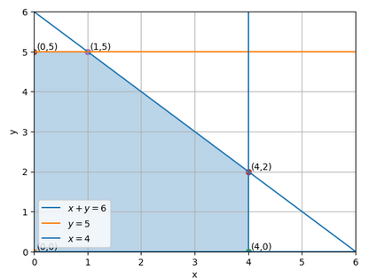
Example (Vertex Method – Maximisation)
Maximise
\( \mathrm{Z = 3x + 2y} \)
subject to:
\( \mathrm{x + y \leq 6} \)
\( \mathrm{x \leq 4} \)
\( \mathrm{y \leq 5} \)
\( \mathrm{x \geq 0,\; y \geq 0} \)
▶️ Answer/Explanation
Vertices of feasible region:
\( (0,0), (4,0), (4,2), (1,5), (0,5) \)
Evaluate \( \mathrm{Z} \):
At \( (0,0): Z = 0 \)
At \( (4,0): Z = 12 \)
At \( (4,2): Z = 16 \)
At \( (1,5): Z = 13 \)
At \( (0,5): Z = 10 \)
Conclusion: Maximum value is \( \mathrm{Z = 16} \) at \( \mathrm{(4,2)} \).
Example (Ruler Method – Maximisation)
Maximise
\( \mathrm{Z = 5x + 4y} \)
subject to:
\( \mathrm{2x + y \leq 10} \)
\( \mathrm{x + y \leq 7} \)
\( \mathrm{x \geq 0,\; y \geq 0} \)
▶️ Answer/Explanation
Feasible region vertices:
\( (0,0), (5,0), (3,4), (0,7) \)
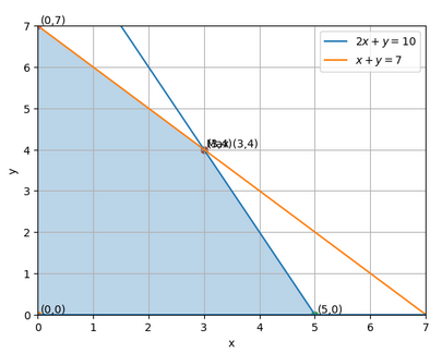
Using ruler method:
Draw \( \mathrm{5x + 4y = k} \) and slide it outwards.
Check vertices:
At \( (5,0): Z = 25 \)
At \( (3,4): Z = 31 \)
At \( (0,7): Z = 28 \)
Conclusion: Maximum value is \( \mathrm{Z = 31} \) at \( \mathrm{(3,4)} \).
Example (Minimisation Problem)
Minimise
\( \mathrm{C = 2x + 3y} \)
subject to:
\( \mathrm{x + 2y \geq 8} \)
\( \mathrm{x + y \geq 5} \)
\( \mathrm{x \geq 0,\; y \geq 0} \)
▶️ Answer/Explanation
Vertices of feasible region:
Intersection of \( x + 2y = 8 \) and \( x + y = 5 \)
Solving gives \( (2,3) \)
Other vertices: \( (0,5), (8,0) \)
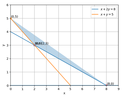
Evaluate \( \mathrm{C} \):
At \( (2,3): C = 13 \)
At \( (0,5): C = 15 \)
At \( (8,0): C = 16 \)
Conclusion: Minimum cost is \( \mathrm{13} \) at \( \mathrm{(2,3)} \).