Solving Equations Numerically by Interval Bisection
Some equations of the form \( f(x) = 0 \) cannot be solved exactly using algebra. In such cases, numerical methods are used to find approximate solutions.
Interval bisection is a simple and reliable method for locating a root.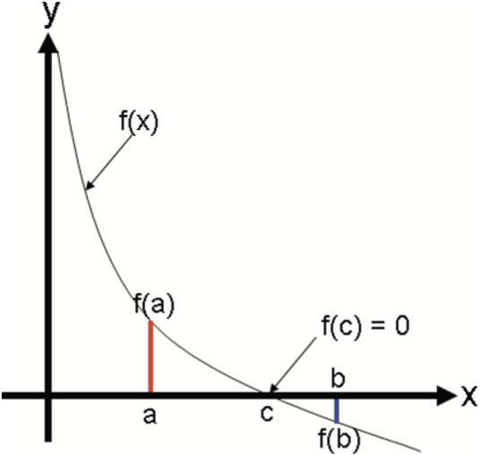
Idea of the Bisection Method
If \( f(x) \) is continuous and:
\( f(a) \) and \( f(b) \) have opposite signs,
then there is at least one root between \( a \) and \( b \).
This follows from the Intermediate Value Theorem.
The bisection method repeatedly halves the interval to locate the root.
Bisection Algorithm
| Step | What to Do |
| 1 | Choose values \( a \) and \( b \) so that \( f(a)f(b) < 0 \). |
| 2 | Find the midpoint \( m = \dfrac{a+b}{2} \). |
| 3 | Evaluate \( f(m) \). |
| 4 | Replace the endpoint that has the same sign as \( f(m) \) with \( m \). |
| 5 | Repeat until the root is found to the required accuracy. |
Example
Use the bisection method to solve \( f(x) = x^3 – x – 2 = 0 \) in the interval \( 1 \le x \le 2 \).
▶️ Answer / Explanation
\( f(1) = 1 – 1 – 2 = -2 \)
\( f(2) = 8 – 2 – 2 = 4 \)
Since the signs are different, a root lies between 1 and 2.
Midpoint:
\( m_1 = \dfrac{1 + 2}{2} = 1.5 \)
\( f(1.5) = 3.375 – 1.5 – 2 = -0.125 \)
The root lies between 1.5 and 2.
Next midpoint:
\( m_2 = \dfrac{1.5 + 2}{2} = 1.75 \)
\( f(1.75) = 5.36 – 1.75 – 2 = 1.61 \)
The root lies between 1.5 and 1.75.
Next midpoint:
\( m_3 = \dfrac{1.5 + 1.75}{2} = 1.625 \)
\( f(1.625) = 4.29 – 1.625 – 2 = 0.665 \)
The root lies between 1.5 and 1.625.
Continuing this process gives:
\( x \approx 1.52 \) (to 2 decimal places)
Solving \( f(x)=0 \) by Linear Interpolation
Linear interpolation is a numerical method used to find an approximate root of an equation when the graph of \( f(x) \) crosses the x-axis between two known values.
It assumes that between two nearby points the graph is approximately a straight line.
Idea Behind Linear Interpolation
If \( f(a) \) and \( f(b) \) have opposite signs, then a root lies between \( a \) and \( b \).
Instead of taking the midpoint as in bisection, linear interpolation joins the points \( (a, f(a)) \) and \( (b, f(b)) \) with a straight line and finds where that line crosses the x-axis.
This usually gives a more accurate estimate than bisection.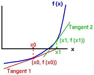
Formula
If \( f(a) \) and \( f(b) \) have opposite signs, the root \( x \) is approximated by:
\( x = a + \dfrac{(b-a)(0 – f(a))}{f(b) – f(a)} \)
or equivalently:
\( x = \dfrac{a f(b) – b f(a)}{f(b) – f(a)} \)
When to Use It
- When \( f(a)f(b) < 0 \).
- When the function is reasonably smooth between \( a \) and \( b \).
- When a faster approximation than bisection is required.
Example
Use linear interpolation to solve \( f(x) = x^3 – x – 2 = 0 \) between \( x = 1 \) and \( x = 2 \).
▶️ Answer / Explanation
\( f(1) = 1 – 1 – 2 = -2 \)
\( f(2) = 8 – 2 – 2 = 4 \)
Use the formula:
\( x = \dfrac{1 \cdot 4 – 2(-2)}{4 – (-2)} \)
\( = \dfrac{4 + 4}{6} = \dfrac{8}{6} = \dfrac{4}{3} \)
\( x \approx 1.33 \)
This is an approximation of the root.
Why It Works
Linear interpolation assumes the graph between \( a \) and \( b \) behaves like a straight line. The intersection of this straight line with the x-axis is taken as the approximate root.
Comparison with Bisection
| Method | How the new value is chosen |
| Bisection | Midpoint of the interval |
| Linear interpolation | x-intercept of the straight line joining the two points |
Solving \( f(x)=0 \) by the Newton–Raphson Method
The Newton–Raphson method is a powerful numerical technique used to find accurate approximations to the roots of an equation of the form:
\( f(x) = 0 \)
It uses the idea of a tangent to the curve to improve an initial estimate of a root.
Geometric Idea
Suppose we have an approximate value \( x_n \) for a root. At this point, we draw the tangent to the curve \( y = f(x) \). Where this tangent meets the x-axis gives a better approximation \( x_{n+1} \).
This process is then repeated.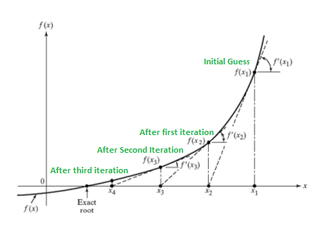
Newton–Raphson Formula
If \( x_n \) is the current approximation, then the next approximation is:
\( x_{n+1} = x_n – \dfrac{f(x_n)}{f'(x_n)} \)
Only differentiation from P1 and P2 is required.
When the Method Works
- \( f(x) \) must be differentiable near the root.
- The starting value must be reasonably close to the root.
- \( f'(x_n) \) must not be zero.
Algorithm
| Step | What to Do |
| 1 | Choose an initial approximation \( x_0 \). |
| 2 | Calculate \( x_1 = x_0 – \dfrac{f(x_0)}{f'(x_0)} \). |
| 3 | Repeat to find \( x_2, x_3, \dots \) until stable. |
Comparison of Numerical Methods
| Method | Speed | Reliability |
| Bisection | Slow | Always works |
| Linear interpolation | Medium | Usually works |
| Newton–Raphson | Fast | Depends on starting value |
Example
Use the Newton–Raphson method to solve \( f(x) = x^3 – x – 2 = 0 \) starting with \( x_0 = 1.5 \).
▶️ Answer / Explanation
\( f(x) = x^3 – x – 2 \)
\( f'(x) = 3x^2 – 1 \)
First iteration:
\( x_1 = 1.5 – \dfrac{1.5^3 – 1.5 – 2}{3(1.5)^2 – 1} \)
\( = 1.5 – \dfrac{3.375 – 3.5}{6.75 – 1} = 1.5 – \dfrac{-0.125}{5.75} \)
\( x_1 \approx 1.5217 \)
Second iteration:
\( x_2 = 1.5217 – \dfrac{(1.5217)^3 – 1.5217 – 2}{3(1.5217)^2 – 1} \)
\( x_2 \approx 1.5214 \)
So the root is approximately:
\( x \approx 1.521 \)