Diagonalisation of \( 2 \times 2 \) Matrices and Applications
Diagonalisation is the process of transforming a matrix into a diagonal matrix using a suitable change of basis. For certain matrices, especially symmetric matrices, this can be done using an orthogonal matrix.
1. What Does Diagonalisation Mean?
A \( 2 \times 2 \) matrix \( A \) is said to be diagonalisable if it can be written in the form
\( A = PDP^{-1} \)
where
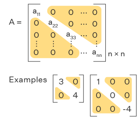
- \( D \) is a diagonal matrix containing the eigenvalues of \( A \)
- the columns of \( P \) are eigenvectors of \( A \)
2. Orthogonal Diagonalisation
If \( A \) is a real symmetric matrix, then its eigenvectors corresponding to distinct eigenvalues are orthogonal. In this case, we can choose normalised eigenvectors to form an orthogonal matrix \( P \).
An orthogonal matrix satisfies
\( P^{\mathrm{T}}P = PP^{\mathrm{T}} = I \)
For orthogonal diagonalisation, the required form is
\( P^{\mathrm{T}} A P = D \)
where \( D \) is diagonal and contains the eigenvalues of \( A \).
3. Steps for Orthogonal Diagonalisation of a \( 2 \times 2 \) Matrix
- Check that \( A \) is symmetric
- Find the eigenvalues of \( A \)
- Find corresponding eigenvectors
- Normalise the eigenvectors
- Form \( P \) using the normalised eigenvectors as columns
- Compute \( P^{\mathrm{T}} A P \)
4. Applications of Diagonalisation
- Simplifying matrix powers such as \( A^n \)
- Understanding stretching along principal directions
- Decoupling systems of linear transformations
Example 1
Diagonalise the matrix
\( A = \begin{pmatrix} 3 & 1 \\ 1 & 3 \end{pmatrix} \)
▶️ Answer / Explanation
Characteristic equation:
\( \begin{vmatrix} 3-\lambda & 1 \\ 1 & 3-\lambda \end{vmatrix} = (3-\lambda)^2 – 1 = 0 \)
Eigenvalues:
\( \lambda = 4,\; 2 \)
Eigenvectors:
For \( \lambda = 4 \): \( \begin{pmatrix}1\\1\end{pmatrix} \), for \( \lambda = 2 \): \( \begin{pmatrix}1\\-1\end{pmatrix} \)
Normalising:
\( \dfrac{1}{\sqrt{2}}\begin{pmatrix}1\\1\end{pmatrix},\; \dfrac{1}{\sqrt{2}}\begin{pmatrix}1\\-1\end{pmatrix} \)
Hence
\( P = \dfrac{1}{\sqrt{2}} \begin{pmatrix} 1 & 1 \\ 1 & -1 \end{pmatrix}, \quad D = \begin{pmatrix} 4 & 0 \\ 0 & 2 \end{pmatrix} \)
Conclusion: \( P^{\mathrm{T}} A P = D \).
Example 2
Verify that the matrix \( P \) in Example 1 diagonalises \( A \).
▶️ Answer / Explanation
Since \( P \) is orthogonal, \( P^{-1} = P^{\mathrm{T}} \).
\( P^{\mathrm{T}}AP = \begin{pmatrix} 4 & 0 \\ 0 & 2 \end{pmatrix} \)
Conclusion: The matrix is diagonal as required.
Example 3
Use diagonalisation to find \( A^3 \) for the matrix in Example 1.
▶️ Answer / Explanation
Using \( A = PDP^{\mathrm{T}} \):
\( A^3 = PD^3P^{\mathrm{T}} \)
Since
\( D^3 = \begin{pmatrix} 64 & 0 \\ 0 & 8 \end{pmatrix} \)
Conclusion: Diagonalisation makes powers of matrices easy to compute.