Graphs of Functions and Sketching Curves
A function is a rule that maps each input \( x \) to exactly one output \( y \). The graph of a function \( y = f(x) \) is a visual representation of all points \((x, f(x))\).
Sketching graphs helps to understand the behaviour of a function, including key features such as intercepts, turning points, asymptotes, and long-term behaviour.
Key Ideas in Sketching Functions
| Feature | Description | Graph |
| Intercepts | x-intercepts: solve \( f(x) = 0 \) y-intercept: \( f(0) \) | 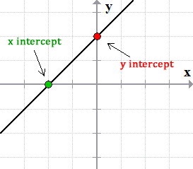 |
| Turning points | Where the graph changes direction (common in quadratics and cubics) | 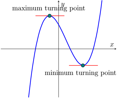 |
| Asymptotes | Lines the graph approaches but never touches (e.g., \( x = 0 \) for \( y = \dfrac{k}{x} \)) |  |
| End behaviour | How the function behaves as \( x \to \infty \) or \( x \to -\infty \) |  |
| Symmetry | Even: symmetric about y-axis Odd: symmetric about origin |  |
Sketching Curves Defined by Simple Equations
Some standard functions appear frequently and must be recognised:
- Linear: \( y = mx + c \)
- Quadratic: \( y = ax^2 + bx + c \) (parabola)
- Cubic: \( y = x^3 \), \( y = ax^3 + bx^2 + cx + d \)
- Reciprocal: \( y = \dfrac{k}{x} \), \( y = \dfrac{k}{x^2} \), with asymptotes at \( x = 0 \)
- Trig graphs: \( y = \sin x,\ y = \cos x,\ y = \tan x \)
Recognising these standard shapes is essential for sketching and solving equations graphically.
Geometrical Interpretation of Algebraic Solutions
Solving equations algebraically corresponds to finding intersection points of graphs.
For example, solving:
\( f(x) = g(x) \)
means finding all \( x \)-values where the graphs of \( y = f(x) \) and \( y = g(x) \) intersect.
Each solution of \( f(x) = g(x) \) is an x-coordinate of an intersection point.
This interpretation helps solve equations visually, check the number of solutions, or understand inequalities.
Using Intersection Points to Solve Equations
| Equation | Graphical Meaning |
| \( f(x) = g(x) \) | Points where graphs intersect |
| \( f(x) > g(x) \) | Region where graph of \( f(x) \) lies above graph of \( g(x) \) |
| \( f(x) < g(x) \) | Region where graph of \( f(x) \) lies below graph of \( g(x) \) |
Example
Find the solution of the equation \( x + 2 = 3x – 4 \) and interpret it graphically.
▶️ Answer / Explanation
Solve algebraically:
\( x + 2 = 3x – 4 \Rightarrow 2x = 6 \Rightarrow x = 3 \)
Graphical meaning:
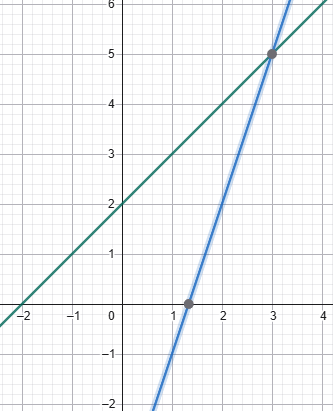
The lines \( y = x + 2 \) and \( y = 3x – 4 \) intersect at \( x = 3 \).
Example
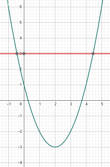
Use a graph to solve the equation \( x^2 – 4x + 1 = 3 \).
▶️ Answer / Explanation
Rewrite:
\( x^2 – 4x + 1 = 3 \Rightarrow x^2 – 4x – 2 = 0 \)
Graphical interpretation:
Intersection of \( y = x^2 – 4x + 1 \) and \( y = 3 \).
Solutions are the x-coordinates where the parabola meets the horizontal line \( y = 3 \).
Algebraic solution:
\( x = 2 \pm \sqrt{3} \)
Example
The functions \( f(x) = x^3 – 2x \) and \( g(x) = \dfrac{4}{x} \) are plotted on the same axes. Find the number of solutions to \( f(x) = g(x) \) using a graphical argument.
▶️ Answer / Explanation
The graph of \( f(x) = x^3 – 2x \) is a cubic passing through the origin with two turning points.
The graph of \( g(x) = \dfrac{4}{x} \) has asymptotes at \( x = 0 \) and \( y = 0 \).
Graphically, the two curves intersect in three places (one in each of two quadrants and one near the origin).
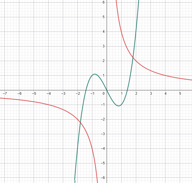
Conclusion: The equation \( x^3 – 2x = \dfrac{4}{x} \) has 3 real solutions.
Graphs of Cubic, Reciprocal, and Trigonometric Functions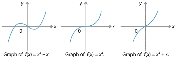
1. Simple Cubic Functions
A simple cubic is a function of the form:
\( y = x^3,\quad y = x^3 + px,\quad y = ax^3 + bx^2 + cx + d \)
Key Features of Cubic Graphs
| Feature | Description |
| Shape | S-shaped curve; passes through origin for simple forms |
| End behaviour | If \( a > 0 \): left ↓, right ↑ If \( a < 0 \): left ↑, right ↓ |
| Turning points | General cubic has at most 2 turning points |
2. Reciprocal Functions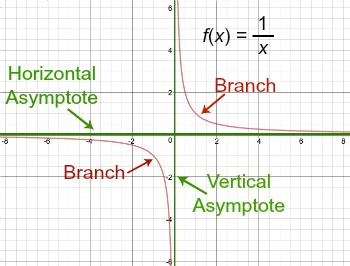
2.1 The function \( y = \dfrac{k}{x} \)
Defined for all \( x \neq 0 \).
Key properties:
- Two symmetrical branches (quadrants I and III when \( k > 0 \))
- Vertical asymptote at \( x = 0 \)
- Horizontal asymptote at \( y = 0 \)
2.2 The function \( y = \dfrac{k}{x^2} \)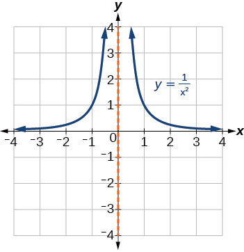
- Defined for all \( x \neq 0 \)
- Always positive when \( k > 0 \)
- Branches in quadrants I and II
- Vertical asymptote: \( x = 0 \)
- Horizontal asymptote: \( y = 0 \)
3. Asymptotes
Definition:
An asymptote is a line that a graph approaches but never touches or crosses as \( x \) or \( y \) becomes very large in magnitude.
Common types:
| Type | Example | Occurs when… |
| Vertical asymptote | \( x = 0 \) for \( y = \dfrac{k}{x} \) | Denominator → 0 |
| Horizontal asymptote | \( y = 0 \) for \( y = \dfrac{k}{x^2} \) | Function → constant as \( |x| \to \infty \) |
4. Trigonometric Graphs
4.1 Graph of \( y = \sin x \)

- Amplitude = 1
- Period = \( 2\pi \)
- Crosses origin
4.2 Graph of \( y = \cos x \)

- Amplitude = 1
- Period = \( 2\pi \)
- Maximum at \( x = 0 \)
4.3 Graph of \( y = \tan x \)

- Period = \( \pi \)
- Vertical asymptotes at \( x = \pm \dfrac{\pi}{2},\ \pm \dfrac{3\pi}{2},\dots \)
- Crosses origin
Example
Sketch the graph of \( y = x^3 \).
▶️ Answer / Explanation
- Passes through origin
- S-shape increasing curve
- As \( x \to -\infty \), \( y \to -\infty \)
- As \( x \to \infty \), \( y \to \infty \)
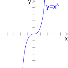
The graph is symmetric about the origin (odd function).
Example
Sketch the reciprocal function \( y = \dfrac{5}{x} \).
▶️ Answer / Explanation
Asymptotes:
\( x = 0 \) and \( y = 0 \)
Behaviour:
- Quadrants I and III (because \( 5 > 0 \))
- Approaches axes but never meets them
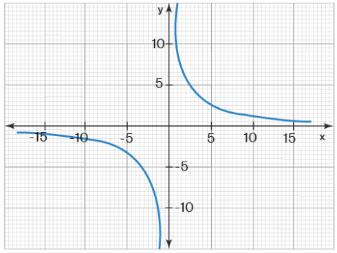
Graph is a smooth decreasing curve in both quadrants.
Example
The curves \( y = 2x^3 – x \) and \( y = \tan x \) are drawn on the same axes. Explain how many intersections they may have.
▶️ Answer / Explanation
Reasoning:
- The cubic is continuous for all real \( x \).
- The \( \tan x \) graph has vertical asymptotes and repeats every \( \pi \).
- Between each pair of asymptotes, the cubic must cross the tan curve at least once.
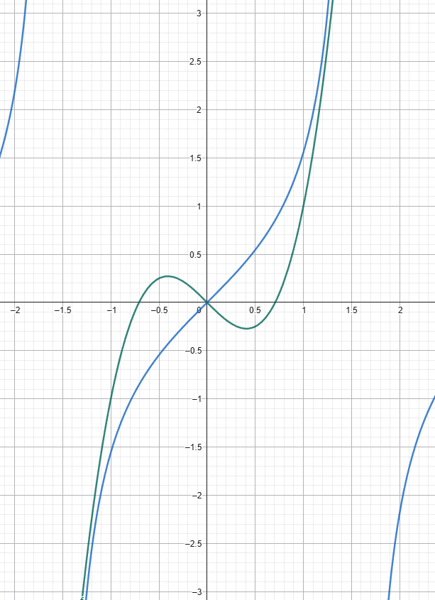
Conclusion: There are infinitely many intersection points — one in each interval \( \left( -\dfrac{\pi}{2} + n\pi,\ \dfrac{\pi}{2} + n\pi \right) \).