Using Logarithmic Graphs to Estimate Parameters
Some relationships are not linear in their original form but can be made linear by taking logarithms.
This allows unknown constants to be estimated using straight-line graphs.
Power Law Model: \( y = ax^n \)
This model is used when one quantity varies as a power of another.
Take logarithms on both sides: 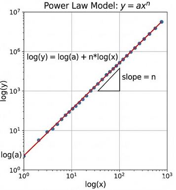
\( \log y = \log a + n\log x \)
This is in the form:
\( Y = c + mX \)
where:
- \( Y = \log y \)
- \( X = \log x \)
- Gradient \( = n \)
- Intercept \( = \log a \)
Graph to Plot
Plot \( \log y \) against \( \log x \)
If the model is correct, the points lie approximately on a straight line.
Finding the Constants
- Gradient of the graph gives \( n \)
- Intercept gives \( \log a \)
- Hence \( a = 10^{\log a} \)
Example (Power Law)
Experimental data suggests that \( y = ax^n \).
A graph of \( \log y \) against \( \log x \) gives a straight line with:
Gradient \( = 1.5 \), intercept \( = 0.3 \)
▶️ Answer / Explanation
\( n = 1.5 \)
\( \log a = 0.3 \Rightarrow a = 10^{0.3} \)
\( a \approx 2.0 \)
Model:
\( y = 2.0x^{1.5} \)
Exponential Model: \( y = kb^x \)
This model is used for exponential growth or decay.
Take logarithms on both sides: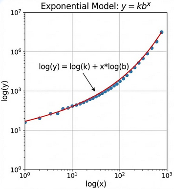
\( \log y = \log k + x\log b \)
This is a linear equation in \( x \).
Graph to Plot
Plot \( \log y \) against \( x \)
If the model is correct, the graph is a straight line.
Finding the Constants
- Gradient \( = \log b \)
- Intercept \( = \log k \)
- \( b = 10^{\text{gradient}} \)
- \( k = 10^{\text{intercept}} \)
Example (Exponential Model)
The relationship between \( x \) and \( y \) is modelled by:
\( y = kb^x \)
A graph of \( \log y \) against \( x \) has:
Gradient \( = 0.04 \), intercept \( = 1.2 \)
▶️ Answer / Explanation
\( \log b = 0.04 \Rightarrow b = 10^{0.04} \)
\( b \approx 1.096 \)
\( \log k = 1.2 \Rightarrow k = 10^{1.2} \)
\( k \approx 15.8 \)
Model:
\( y = 15.8(1.096)^x \)
Choosing the Correct Graph
| Model | Graph to Plot |
| \( y = ax^n \) | \( \log y \) vs \( \log x \) |
| \( y = kb^x \) | \( \log y \) vs \( x \) |
Example: Logarithmic Graphs and Model Identification
Experimental data relating variables \( x \) and \( y \) is analysed.
It is found that a plot of \( \log y \) against \( \log x \) produces a straight line with:
Gradient \( = 2.3 \)
Intercept \( = -0.4 \)
(a) State the form of the relationship between \( x \) and \( y \).
(b) Find the equation connecting \( x \) and \( y \).
▶️ Answer / Explanation
(a) Identifying the model
Since a straight line is obtained by plotting \( \log y \) against \( \log x \), the model is:
\( y = ax^n \)
(b) Finding the constants
From the linearised equation:
\( \log y = \log a + n\log x \)
Comparing with the straight-line graph:
- \( n = 2.3 \)
- \( \log a = -0.4 \)
So:
\( a = 10^{-0.4} \approx 0.40 \)
Final model:
\( \boxed{y = 0.40x^{2.3}} \)