Exponential Growth
Exponential growth occurs when the rate of increase of a quantity is proportional to its current value.
This type of growth is commonly used to model populations, investments, and biological growth.
Basic Exponential Growth Model
The general form of an exponential growth model is: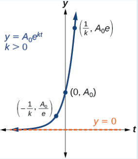
\( y = Ae^{kt} \)
where:
- \( y \) is the quantity at time \( t \)
- \( A \) is the initial value
- \( k > 0 \) is the growth constant
- \( t \) represents time
Meaning of “Initial Value”
The initial value is the value of the quantity when:
\( t = 0 \)
Substituting \( t = 0 \) into the model:
\( y = Ae^{k(0)} = A \)
This confirms that \( A \) is the initial amount.
Rate of Growth
Differentiate \( y = Ae^{kt} \) with respect to \( t \):
\( \dfrac{dy}{dt} = kAe^{kt} = ky \)
This shows that the rate of growth is proportional to the current value of \( y \).
Growth Using Bases Other Than \( e \)
Exponential growth may also be written as:
\( y = a^x \)
The derivative is:
\( \dfrac{d}{dx}(a^x) = a^x \ln a \)
This result is essential when differentiating exponential models with base \( a \).
Graphical Behaviour
- The graph increases continuously
- The curve becomes steeper as \( t \) increases
- The y-intercept is the initial value
- The function has no maximum value
Behaviour for Large Values of \( t \)
As \( t \to \infty \):
\( y = Ae^{kt} \to \infty \)
This may become unrealistic in real-world situations due to limitations such as resources or space.
Validity of the Model
Exponential growth models are usually valid only for a limited range of values of \( t \).
For very large values of \( t \), predictions may become unrealistic.
In such cases, an improved model may be required.
Improved Model (Conceptual)
An improved model may:
- Restrict the domain of \( t \)
- Include limiting factors
- Use a different functional form
This ensures predictions remain physically meaningful.
Example
A quantity grows according to:
\( y = 5e^{0.3t} \)
State the initial value.
▶️ Answer / Explanation
The initial value occurs when \( t = 0 \):
\( y = 5e^0 = 5 \)
Initial value: \( 5 \)
Example
A population is modelled by:
\( P = 200e^{0.05t} \)
Find the rate of growth when \( t = 4 \).
▶️ Answer / Explanation
Differentiate:
\( \dfrac{dP}{dt} = 200(0.05)e^{0.05t} = 10e^{0.05t} \)
At \( t = 4 \):
\( \dfrac{dP}{dt} = 10e^{0.2} \)
Example
A quantity is modelled by:
\( y = 3(1.2)^t \)
Find \( \dfrac{dy}{dt} \) in terms of \( t \).
▶️ Answer / Explanation
Use the result:
\( \dfrac{d}{dt}(a^t) = a^t \ln a \)
\( \dfrac{dy}{dt} = 3(1.2)^t \ln(1.2) \)
Exponential Decay
Exponential decay occurs when the rate of decrease of a quantity is proportional to its current value.
This type of model is commonly used for radioactive decay, cooling, depreciation, and drug concentration in the body.
Basic Exponential Decay Model
The general form of an exponential decay model is: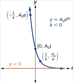
\( y = Ae^{kt} \)
where:
- \( y \) is the quantity at time \( t \)
- \( A \) is the initial value
- \( k < 0 \) is the decay constant
- \( t \) represents time
Initial Value
The initial value is the value of the quantity when:
\( t = 0 \)
Substitute \( t = 0 \):
\( y = Ae^{0} = A \)
Rate of Decay
Differentiate \( y = Ae^{kt} \) with respect to \( t \):
\( \dfrac{dy}{dt} = kAe^{kt} = ky \)
This shows that the rate of change is negative and proportional to the current value.
Decay Using Bases Other Than \( e \)
Exponential decay may also be written as:
\( y = a^x \quad \text{where } 0<a<1 \)
The derivative is:
\( \dfrac{d}{dx}(a^x) = a^x \ln a \)
Since \( \ln a < 0 \), the derivative is negative, confirming decay.
Graphical Behaviour
- The graph decreases continuously
- The curve becomes flatter as \( t \) increases
- The y-intercept is the initial value
- The function never reaches zero
Behaviour for Large Values of \( t \)
As \( t \to \infty \):
\( y = Ae^{kt} \to 0 \)
The quantity approaches zero but never becomes negative.
Validity and Improved Models
Exponential decay models are usually valid only over a limited time interval.
For very small values of the quantity, predictions may no longer be realistic.
An improved model may:
- Restrict the domain of \( t \)
- Introduce a minimum threshold value
- Use piecewise modelling
Example
A substance decays according to:
\( y = 80e^{-0.4t} \)
State the initial amount.
▶️ Answer / Explanation
At \( t = 0 \):
\( y = 80e^0 = 80 \)
Initial amount: \( 80 \)
Example
A quantity is modelled by:
\( y = 150e^{-0.2t} \)
Find the rate of decrease when \( t = 5 \).
▶️ Answer / Explanation
Differentiate:
\( \dfrac{dy}{dt} = -0.2(150)e^{-0.2t} = -30e^{-0.2t} \)
At \( t = 5 \):
\( \dfrac{dy}{dt} = -30e^{-1} \)
Example
The mass \( m \) grams of a radioactive substance after \( t \) hours is modelled by:
\( m = 500(0.85)^t \)
(a) State the initial mass.
(b) Find \( \dfrac{dm}{dt} \).
(c) Comment on the suitability of this model for very large values of \( t \).
▶️ Answer / Explanation
(a) Initial mass
At \( t = 0 \):
\( m = 500(0.85)^0 = 500 \)
(b) Rate of decay
Use:
\( \dfrac{d}{dt}(a^t) = a^t\ln a \)
\( \dfrac{dm}{dt} = 500(0.85)^t\ln(0.85) \)
Since \( \ln(0.85)<0 \), the mass is decreasing.
(c) Suitability of the model
As \( t \to \infty \), \( m \to 0 \).
In reality, measurements become unreliable for very small masses, so the model may only be valid over a limited time interval.