Measures of Location
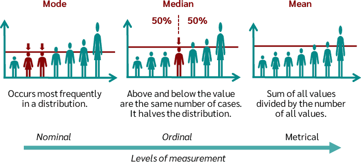
Measures of location describe the central or typical value of a data set. The three most common measures of location are the mean, median, and mode. These measures are used to summarise data and to compare different data sets.
Types of Data
In this syllabus, data may be:
- Discrete data: values that can be counted (e.g. number of students)
- Continuous data: values that can take any value in an interval (e.g. height, time)
- Ungrouped data: raw data values listed individually
- Grouped data: data organised into class intervals
Mean
The mean is the arithmetic average of the data values.
For ungrouped data \( x_1, x_2, \dots, x_n \), the mean is
\( \bar{x} = \dfrac{x_1 + x_2 + \cdots + x_n}{n} \)
The mean uses all values in the data set, but it can be affected by extreme values (outliers).
Median
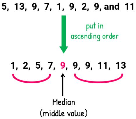
The median is the middle value when the data are arranged in ascending or descending order.
If the number of observations is:
- Odd: the median is the central value
- Even: the median is the mean of the two central values
The median is not affected by extreme values and is useful for skewed data.
Mode
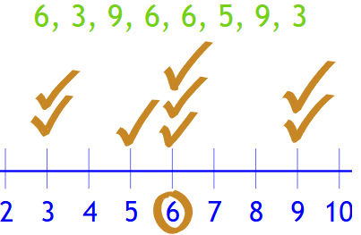
The mode is the value that occurs most frequently in a data set.
A data set may be:
- Unimodal: one mode
- Bimodal: two modes
- Multimodal: more than two modes
The mode is especially useful for categorical or discrete data.
Measures of Dispersion (Overview)
Measures of dispersion describe how spread out the data values are.
| Measure | Description |
|---|---|
| Range | Difference between the largest and smallest values |
| Interquartile range (IQR) | Difference between the upper and lower quartiles |
Although direct calculation will not usually be examined, students must be able to interpret these measures and compare distributions.
Understanding and Use of Coding
Coding is used to simplify calculations by transforming data values.
If a new variable \( y \) is defined by
\( y = \dfrac{x – a}{b} \)
then:
The mean of \( y \) can be found more easily
The mean of \( x \) can then be recovered from the coded mean
Coding does not change the shape of the distribution, only its scale and position.
Interpretation and Inference
Students are expected to:
- Compare distributions using measures of location and dispersion
- Comment on skewness using mean and median
- Interpret results in context
Formal significance tests are not required in this syllabus.
Example :
Two data sets A and B have the same mean of 60. Data set A has an interquartile range of 12, while data set B has an interquartile range of 25. Compare the two data sets.
▶️ Answer/Explanation
Both data sets have the same mean, so they have the same average value.
However, data set B has a larger interquartile range.
This means the middle 50% of the data in B is more spread out
Conclusion: Data set A is more consistent, while data set B shows greater variability.
Example :
The mean score of a test is 68, while the median score is 74. Describe the likely shape of the distribution.
▶️ Answer/Explanation
The mean is less than the median.
This suggests that some lower values are pulling the mean down.
The distribution is therefore negatively skewed (skewed to the left)
Conclusion: Most students scored relatively highly, with a few low scores.
Example :
In a factory, the mode of the number of items produced per hour is 120. Explain why the mode is an appropriate measure of location in this context.
▶️ Answer/Explanation
The mode represents the most frequently occurring value.
In a production setting:
The most common output per hour is often of greatest practical interest
Extreme values are less important than typical performance
Conclusion: The mode gives a clear indication of the usual hourly production.