The Normal Distribution
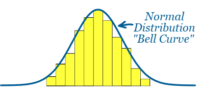
The normal distribution is a continuous probability distribution that is widely used to model real-life data such as heights, weights, measurement errors, and examination marks.
A random variable that follows a normal distribution is written as
\( X \sim N(\mu, \sigma^2) \)
where:
\( \mu \) is the mean
\( \sigma^2 \) is the variance
\( \sigma \) is the standard deviation
Shape and Symmetry
The normal distribution has the following key features:
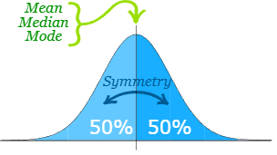
- It is symmetric about the mean \( \mu \)
- The mean, median, and mode are equal
- The curve is bell-shaped
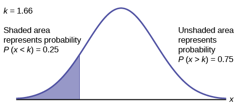
Because of the symmetry, probabilities on either side of the mean are equal.
Mean and Variance
For a normally distributed random variable \( X \sim N(\mu, \sigma^2) \):
\( E(X) = \mu \)
\( \mathrm{Var}(X) = \sigma^2 \)
These results may be used directly without proof.
Standardisation
Probabilities for the normal distribution are found by converting values of \( X \) to a standard normal variable \( Z \), where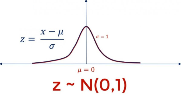
\( Z = \dfrac{X – \mu}{\sigma} \)
The standard normal distribution is written as
\( Z \sim N(0,1) \)
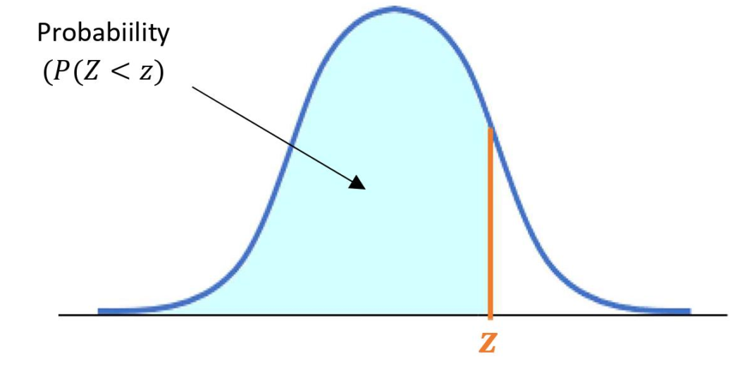
Use of Normal Distribution Tables
Tables give values of the cumulative distribution function
\( P(Z \leq z) \)
To find probabilities involving \( X \):
- Convert values of \( X \) to \( Z \) using standardisation
- Use the table to find probabilities for \( Z \)
- Use symmetry when appropriate
Interpolation is not required in this syllabus.
Z- table value:
| z | 0.00 | 0.01 | 0.02 | 0.03 | 0.04 | 0.05 | 0.06 | 0.07 | 0.08 | 0.09 |
|---|---|---|---|---|---|---|---|---|---|---|
| 0.0 | 0.5000 | 0.5040 | 0.5080 | 0.5120 | 0.5160 | 0.5199 | 0.5239 | 0.5279 | 0.5319 | 0.5359 |
| 0.1 | 0.5398 | 0.5438 | 0.5478 | 0.5517 | 0.5557 | 0.5596 | 0.5636 | 0.5675 | 0.5714 | 0.5754 |
| 0.2 | 0.5793 | 0.5832 | 0.5871 | 0.5910 | 0.5948 | 0.5987 | 0.6026 | 0.6064 | 0.6103 | 0.6141 |
| 0.3 | 0.6179 | 0.6217 | 0.6255 | 0.6293 | 0.6331 | 0.6368 | 0.6406 | 0.6443 | 0.6480 | 0.6517 |
| 0.4 | 0.6554 | 0.6591 | 0.6628 | 0.6664 | 0.6700 | 0.6736 | 0.6772 | 0.6808 | 0.6844 | 0.6879 |
| 0.5 | 0.6915 | 0.6950 | 0.6985 | 0.7019 | 0.7054 | 0.7088 | 0.7123 | 0.7157 | 0.7190 | 0.7224 |
| 0.6 | 0.7258 | 0.7291 | 0.7324 | 0.7357 | 0.7389 | 0.7422 | 0.7454 | 0.7486 | 0.7518 | 0.7549 |
| 0.7 | 0.7580 | 0.7611 | 0.7642 | 0.7673 | 0.7704 | 0.7734 | 0.7764 | 0.7794 | 0.7823 | 0.7852 |
| 0.8 | 0.7881 | 0.7910 | 0.7939 | 0.7967 | 0.7995 | 0.8023 | 0.8051 | 0.8078 | 0.8106 | 0.8133 |
| 0.9 | 0.8159 | 0.8186 | 0.8212 | 0.8238 | 0.8264 | 0.8289 | 0.8315 | 0.8340 | 0.8365 | 0.8389 |
| 1.0 | 0.8413 | 0.8438 | 0.8461 | 0.8485 | 0.8508 | 0.8531 | 0.8554 | 0.8577 | 0.8599 | 0.8621 |
| 1.1 | 0.8643 | 0.8665 | 0.8686 | 0.8708 | 0.8729 | 0.8749 | 0.8770 | 0.8790 | 0.8810 | 0.8830 |
| 1.2 | 0.8849 | 0.8869 | 0.8888 | 0.8907 | 0.8925 | 0.8944 | 0.8962 | 0.8980 | 0.8997 | 0.9015 |
| 1.3 | 0.9032 | 0.9049 | 0.9066 | 0.9082 | 0.9099 | 0.9115 | 0.9131 | 0.9147 | 0.9162 | 0.9177 |
| 1.4 | 0.9192 | 0.9207 | 0.9222 | 0.9236 | 0.9251 | 0.9265 | 0.9279 | 0.9292 | 0.9306 | 0.9319 |
| 1.5 | 0.9332 | 0.9345 | 0.9357 | 0.9370 | 0.9382 | 0.9394 | 0.9406 | 0.9418 | 0.9430 | 0.9441 |
| 1.6 | 0.9452 | 0.9463 | 0.9474 | 0.9485 | 0.9495 | 0.9505 | 0.9515 | 0.9525 | 0.9535 | 0.9545 |
| 1.7 | 0.9554 | 0.9564 | 0.9573 | 0.9582 | 0.9591 | 0.9599 | 0.9608 | 0.9616 | 0.9625 | 0.9633 |
| 1.8 | 0.9641 | 0.9649 | 0.9656 | 0.9664 | 0.9671 | 0.9678 | 0.9686 | 0.9693 | 0.9700 | 0.9706 |
| 1.9 | 0.9713 | 0.9719 | 0.9726 | 0.9732 | 0.9738 | 0.9744 | 0.9750 | 0.9756 | 0.9761 | 0.9767 |
| 2.0 | 0.9773 | 0.9778 | 0.9783 | 0.9788 | 0.9793 | 0.9798 | 0.9803 | 0.9808 | 0.9812 | 0.9817 |
Using Symmetry
For the standard normal distribution:
\( P(Z \leq 0) = 0.5 \)
\( P(Z \leq -z) = 1 – P(Z \leq z) \)
These properties are frequently used to simplify calculations.
Solving Problems Involving Equations
Some questions may require:
- Finding unknown values of \( \mu \) or \( \sigma \)
- Solving simultaneous equations involving probabilities
These problems rely on correct use of standardisation and normal tables, not on derivation of formulas.
Example :
The mass of packets of rice is normally distributed with mean \( \mu = 5 \) kg and standard deviation \( \sigma = 0.2 \) kg.
Find the probability that a randomly selected packet has a mass less than 4.8 kg.
▶️ Answer/Explanation
Let \( X \sim N(5, 0.2^2) \).
Standardise:
\( Z = \dfrac{4.8 – 5}{0.2} = -1 \)
Using normal tables:
\( P(Z \leq -1) = 1 – P(Z \leq 1) = 1 – 0.8413 = 0.1587 \)
Conclusion: The required probability is 0.1587.
Example :
The heights of students in a college are normally distributed with mean \( \mu = 170 \) cm and standard deviation \( \sigma = 6 \) cm.
Find the probability that a randomly selected student has a height between 164 cm and 176 cm.
▶️ Answer/Explanation
Let \( X \sim N(170, 6^2) \).
Standardise both values:
\( Z_1 = \dfrac{164 – 170}{6} = -1,\quad Z_2 = \dfrac{176 – 170}{6} = 1 \)
Using normal tables and symmetry:
\( P(-1 \leq Z \leq 1) = 0.8413 – 0.1587 = 0.6826 \)
Conclusion: The required probability is 0.6826.
Example :
A random variable \( X \) is normally distributed. It is given that
\( P(X \leq 50) = 0.5 \) and \( P(X \leq 58) = 0.9772 \).
Find the mean \( \mu \) and the standard deviation \( \sigma \).
▶️ Answer/Explanation
Since \( P(X \leq 50) = 0.5 \), the value 50 corresponds to the mean.
\( \mu = 50 \)
From normal tables,
\( P(Z \leq 2) = 0.9772 \)
So,
\( \dfrac{58 – 50}{\sigma} = 2 \)
\( \sigma = 4 \)
Conclusion: The distribution is \( X \sim N(50, 4^2) \).